The majorizing measures theorem

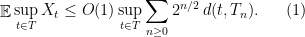
We will now prove Talagrand’s majorizing measures theorem, showing that the generic chaining bound is tight for Gaussian processes. The proof here will be a bit more long-winded than the proof from Talagrand’s book, but also (I think), a bit more accessible as well. Most importantly, we will highlight the key idea with a simple combinatorial argument.

First, let’s recall the bound we proved earlier.

Theorem 1 Let ${\{X_t\}_{t \in T}}$ be a Gaussian process, and let ${T_0 \subseteq T_1 \subseteq \cdots \subseteq T}$ be a sequence of subsets such that ${|T_0|=1}$ and ${|T_n| \leq 2^{2^{n}}}$ for ${n \geq 1}$ . Then,

$\displaystyle \mathop{\mathbb E}\sup_{t \in T} X_t \leq O(1) \sup_{t \in T} \sum_{n \geq 0} 2^{n/2} \, d(t, T_n). \ \ \ \ \ (1)$

In order to make things slightly easier to work with, we look at an essentially equivalent way to state (1). Consider a Gaussian process ${\{X_t\}_{t \in T}}$ and a sequence of increasing partitions ${\{\mathcal A_n\}_{n \geq 0}}$ of ${T}$ , where increasing means that ${\mathcal A_{n+1}}$ is a refinement of ${\mathcal A_n}$ for ${n \geq 0}$ . Say that such a sequence ${\{\mathcal A_n\}}$ is admissible if ${\mathcal A_0 = \{T\}}$ and ${|\mathcal A_n| \leq 2^{2^n}}$ for all ${n \geq 1}$ . Also, for a partition ${P}$ and a point ${t \in T}$ , we will use the notation ${P(t)}$ for the unique set in ${P}$ which contains ${t}$ .

By choosing ${T_n}$ to be any set of points with one element in each piece of the partition ${\mathcal A_n}$ , (1) yields,

$\displaystyle \mathop{\mathbb E}\sup_{t \in T} X_t \leq O(1) \sup_{t \in T} \sum_{n \geq 0} 2^{n/2} \,\mathrm{diam}(\mathcal A_n(t)). \ \ \ \ \ (2)$

We can now state our main theorem, which shows that this is essentially the only way to bound ${\mathop{\mathbb E} \sup_{t \in T} X_t}$ .

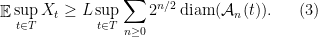
Theorem 2 There is a constant ${L > 0}$ such that for any Gaussian process ${\{X_t\}_{t \in T}}$ , there exists an admissible sequence ${\{\mathcal A_n\}}$ which satisfies,

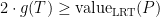
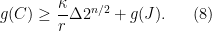
$\displaystyle \mathop{\mathbb E} \sup_{t \in T} X_t \geq L \sup_{t \in T} \sum_{n \geq 0} 2^{n/2} \,\mathrm{diam}(\mathcal A_n(t)). \ \ \ \ \ (3)$

Recall that for a subset ${A \subseteq T}$ , we defined ${g(A) = \mathop{\mathbb E} \sup_{t \in A} X_t}$ , and in the last post, we proved the following “Sudakov inequality.”

Theorem 3 For some constants ${\kappa > 0}$ and ${r \geq 4}$ , the following holds. Suppose ${\{X_t\}_{t \in T}}$ is a Gaussian process, and let ${t_1, t_2, \ldots, t_m \in T}$ be such that ${d(t_i,t_j) \geq \alpha}$ for ${i \neq j}$ . Then,

$\displaystyle g(T) \geq \kappa \alpha \sqrt{\log_2 m} + \min_{i=1,2,\ldots,m} g(B(t_i, \alpha/r)). \ \ \ \ \ (4)$

We will use only Theorem 3 and the fact that ${g(A) \leq g(B)}$ whenever ${A \subseteq B}$ to prove Theorem 2 (so, in fact, Theorem 2 holds with ${\mathop{\mathbb E} \sup_{t \in T} X_t}$ replaced by more general functionals satisfying an inequality like (4)).

The partitioning scheme

First, we will specify the partitioning scheme to form an admissible sequence ${\{\mathcal A_n\}}$ , and then we will move on to its analysis. As discussed in earlier posts, we may assume that ${T}$ is finite. Every set ${C \in \mathcal A_n}$ will have a value ${\mathrm{rad}(C)}$ associated with it, such that ${\mathrm{rad}(C)}$ is always an upper bound on the radius of the set ${C}$ , i.e. there exists a point ${x \in C}$ such that ${C \subseteq B(x, \mathrm{rad}(C))}$ .

Initially, we set ${\mathcal A_0 = \{T\}}$ and ${\mathrm{rad}(T) = \mathrm{diam}(T)}$ . Now, we assume that we have constructed ${\mathcal A_n}$ , and show how to form the partition ${\mathcal A_{n+1}}$ . To do this, we will break every set ${C \in \mathcal A_n}$ into at most ${2^{2^n}}$ pieces. This will ensure that

$\displaystyle |\mathcal A_{n+1}| \leq 2^{2^n} \cdot |\mathcal A_n| \leq 2^{2^n} \cdot 2^{2^n} = 2^{2^{n+1}}.$

Let ${r}$ be the constant from Theorem 3. Put ${m = 2^{2^n}}$ , and let ${\Delta = \mathrm{rad}(C)}$ . We partition ${C}$ into ${m}$ pieces as follows. First, choose ${t_1 \in C}$ which maximizes the value

$\displaystyle g(B(t_1, \Delta/r^2) \cap C).$

Then, set ${C_1 = B(t_1, \Delta/r) \cap C}$ . We put ${\mathrm{rad}(C_1) = \Delta/r}$ .

A remark: The whole idea here is that we have chosen the “largest possible piece,” (in terms of ${g}$ -value), but we have done this with respect to the ${\Delta/r^2}$ ball, while we cut out the ${\Delta/r}$ ball. The reason for this will not become completely clear until the analysis, but we can offer a short explanation here. Looking at the lower bound (4), observe that the balls ${B(t_i, \alpha/3)}$ are disjoint under the assumptions, but we only get “credit” for the ${B(t_i, \alpha/r)}$ balls. When we apply this lower bound, it seems that we are throwing a lot of the space away. At some point, we will have to make sure that this thrown away part doesn’t have all the interesting stuff! The reason for our choice of ${\Delta/r}$ vs. ${\Delta/r^2}$ is essentially this: We want to guarantee that if we miss the interesting stuff at this level, then the previous level took care of it. To have this be the case, we will have to look forward (a level down), which (sort of) explains our choice of optimizing for the ${\Delta/r^2}$ ball.

Now we continue in this fashion. Let ${D_{\ell} = C \setminus \bigcup_{i=1}^{\ell-1} C_i}$ be the remaining space after we have cut out ${\ell-1}$ pieces. For ${\ell \leq m}$ , choose ${t_{\ell} \in C}$ to maximize the value

$\displaystyle g(B(t_{\ell}, \Delta/r^2) \cap D_{\ell}).$

For ${\ell < m}$ , set ${C_{\ell} = B(t_{\ell}, \Delta/r) \cap D_{\ell}}$ , and put ${\mathrm{rad}(C_{\ell}) = \Delta/r}$ .

So far, we have been chopping the space into smaller pieces. If ${D_{\ell} = \emptyset}$ for some ${\ell \leq m}$ , we have finished our construction of ${\mathcal A_{n+1}}$ . But maybe we have already chopped out ${m-1}$ pieces, and still some remains. In that case, we put ${C_m = D_m}$ , i.e. we throw everything else into ${C_m}$ . Since we cannot reduce our estimate on the radius, we also put ${\mathrm{rad}(C_m) = \Delta}$ .

We continue this process until ${T}$ is exhausted, i.e. eventually for some ${n}$ large enough, ${\mathcal A_n}$ only contains singletons. This completes our description of the partitioning.

The tree

For the analysis, it will help to consider our partitioning process as having constructed a tree (in the most natural way). The root of the the tree is the set ${T}$ , and its children are the sets of ${\mathcal A_1}$ , and so on. Let’s call this tree ${\mathcal W}$ . It will help to draw and describe ${\mathcal W}$ in a specific way. First, we will assign values to the edges of the tree. If ${C \in \mathcal A_n}$ and ${C_j}$ is a child of ${C}$ (i.e., ${C_j \in \mathcal A_{n+1}}$ and ${C_j \subseteq C}$ ), then the edge ${(C,C_j)}$ is given value:

$\displaystyle \kappa \cdot \frac{\mathrm{rad}(C)}{r} \cdot 2^{n/2}, \ \ \ \ \ (5)$

where ${\kappa}$ and ${r}$ are the constants from Theorem 3.

If we define the value of a root-leaf path in ${\mathcal W}$ as the sum of the edge lengths on that path, then for any ${t \in T}$ ,

$\displaystyle \sum_{n \geq 0} 2^{n/2}\,\mathrm{diam}(\mathcal A_n(t)) \leq 2 \frac{r}{\kappa} \left(\textrm{value of the path from the root to } t\right),$

simply using ${\mathrm{diam}(\mathcal A_n(t)) \leq 2\, \mathrm{rad}(\mathcal A_n(t))}$ .

Thus in order to prove Theorem 2, which states that for some ${L > 0}$ ,

$\displaystyle g(T) \geq L \sup_{t \in T} \sum_{n \geq 0} 2^{n/2}\,\mathrm{diam}(\mathcal A_n(t)),$

it will suffice to show that for some (other) constant ${L > 0}$ , for any root-leaf path ${P}$ in ${\mathcal W}$ , we have

$\displaystyle g(T) \geq L \cdot \mathrm{value}(P). \ \ \ \ \ (6)$

Before doing this, we will fix a convention for drawing parts of ${\mathcal W}$ . If a node ${C \in \mathcal A_n}$ has children ${C_1, C_2, \ldots, C_m}$ , we will draw them from left to right. We will call an edge ${(C,C_m)}$ a right turn and every other edge will be referred to as a left turn. Note that some node ${C}$ may not have any right turn coming out of it (if the partitioning finished before the last step). Also, observe that along a left turn, the radius always drops by a factor of ${r}$ , while along a right turn, it remains the same.

We now make two observations about computing the value ${\mathrm{value}(P)}$ up to a universal constant.

Observation (1): In computing the value of a root-leaf path ${P}$ , we only need to consider right turns.

To see this, suppose that we have a right turn followed by a consecutive sequence of left turns. If the value of the right turn is ${\frac{\kappa}{r} \Delta 2^{n/2}}$ , then the value of the following sequence of left turns is, in total, at most

$\displaystyle \frac{\kappa}{r} \sum_{j=1}^{\infty} 2^{(n+j)/2} \frac{\Delta}{r^j} \leq O(1) \frac{\kappa}{r} \Delta 2^{n/2}.$

In other words, because the radius decreases by a factor of ${r}$ along every left turn, their values decrease geometrically, making the whole sum comparable to the preceding right turn. (Recall that ${r \geq 4}$ , so indeed the sum is geometric.)

If the problem of possibly of having no right turn in the path ${P}$ bothers you, note that we could artificially add an initial right turn into the root with value ${\mathrm{diam}(T)}$ . This is justified since ${g(T) \geq \frac12 \mathrm{diam}(T)}$ always holds. A different way of saying this is that if the path really contained no right turn, then its value is ${O(\mathrm{diam}(T))}$ , and we can easily prove (6).

Observation (2): In computing the value of a root-leaf path ${P}$ , we need only consider the last right turn in any consecutive sequence of right turns.

Consider a sequence of consecutive right turns, and the fact that the radius does not decrease. The values (taking away the ${\kappa/r}$ factor) look like ${\Delta 2^{n/2}, \Delta 2^{(n+1)/2}, \Delta 2^{(n+2)/2}, \ldots}$ . In other words, they are geometrically increasing, and thus using only the last right turn in every sequence, we only lose a constant factor.

We will abbreviate last right turn to LRT, and write ${\mathrm{value}_{\mathrm{LRT}}(P)}$ to denote the value of ${P}$ , just counting last right turns. By the two observations, to show (6) (and hence finish the proof), it suffices to show that, for every root-leaf path ${P}$ in ${\mathcal W}$ ,

$\displaystyle 2 \cdot g(T) \geq \mathrm{value}_{\mathrm{LRT}}(P). \ \ \ \ \ (7)$

The analysis

Recall that our tree ${\mathcal W}$ has values on the edges, defined in (5). We will also put some natural values on the nodes. For a node ${C}$ (which, recall, is just a subset ${C \subseteq T}$ ), we put ${\mathrm{value}(C) = g(C)}$ . So the edges have values and the nodes have values. Thus given any subset of nodes and edges in ${\mathcal W}$ , we can talk about the value of the subset, which will be the sum of the values of the objects it contains. We will prove (7) by a sequence of inequalities on subsets.

Fix a root-leaf path ${P}$ , for which we will prove (7). Let’s prove the fundamental inequality now. We will consider two consecutive LRTs along ${P}$ . (If there is only one LRT in ${P}$ , then we are done by the preceding remarks.) See the figure below. The dashed lines represent a (possibly empty) sequence of left turns and then right turns. The two LRTs are marked.

We will prove the following inequality, which is the heart of the proof. One should understand that the inequality is on the values of the subsets marked in red. The first subset contains two nodes, and the second contains two nodes and an edge.

With this inequality proved, the proof is complete. Let’s see why. We start with the first LRT. Since $g(T) \geq g(C)$ for any node $C$ in $\mathcal W$ , we have the inequality:

This gets us started. Now we apply the inequality of Figure A repeatedly to each pair of consecutive LRTs in the path ${P}$ . What do we have when we’ve exhausted the path $P$ ? Well, precisely all the LRTs in ${P}$ are marked, yielding ${2 \cdot g(T) \geq \mathrm{value}_{\mathrm{LRT}}(P)}$ , as desired.

The LRT inequality

Now we are left to prove the inequality in Figure A. First, let’s label some of the nodes. Let ${\Delta = \mathrm{rad}(C)}$ , and suppose that ${C \in \mathcal A_n}$ . The purple values are not the radii of the corresponding nodes, but they are upper bounds on the radii, recalling that along every left turn, the radius decreases by a factor of ${r}$ . Since there are at least two left turns in the picture, we get a ${\Delta/r^2}$ upper bound on the radius of ${J}$ .

Part of the inequality is easy: We have ${g(A) \geq g(B)}$ since ${B \subseteq A}$ . So we can transfer the red mark from ${A}$ to ${B}$ . We are thus left to prove that

$\displaystyle g(C) \geq \frac{\kappa}{r} \Delta 2^{n/2} + g(J). \ \ \ \ \ (8)$

This will allow us to transfer the red mark from ${C}$ to the LRT coming out of ${C}$ and to ${J}$ .

When ${C}$ was partitioned into ${m = 2^{2^n}}$ pieces, this was by our greedy partitioning algorithm using centers ${t_1, t_2, \ldots, t_m}$ . Since we cut out the ${\Delta/r}$ ball around each center, we have ${d(t_i, t_j) \geq \Delta/r}$ for all ${i \neq j}$ . Applying the Sudakov inequality (Theorem 3), we have

$\displaystyle \begin{array}{rl} g(C) &\displaystyle \geq \kappa \frac{\Delta}{r} \sqrt{\log_2 m} + \min_{i=1,\ldots,m} g(B(t_i, \Delta/r^2)) \\ \\ &\displaystyle = \frac{\kappa}{r} \Delta 2^{n/2} + \min_{i=1,\ldots,m} g(B(t_i, \Delta/r^2)) \\ \\ &\displaystyle \geq \frac{\kappa}{r} \Delta 2^{n/2} + \min_{i=1,\ldots,m} g(B(t_i, \Delta/r^2) \cap D_i) \\ \\ &\displaystyle = \frac{\kappa}{r} \Delta 2^{n/2} + g(B(t_m, \Delta/r^2) \cap D_m), \\ \end{array}$

where the last line follows from the greedy manner in which the ${t_i}$ ‘s were chosen.

But now we claim that

$\displaystyle g(B(t_m, \Delta/r^2) \cap D_m) \geq g(J). \ \ \ \ \ (9)$

This follows from two facts. First, ${J \subseteq D_m}$ (since ${D_m=C_m}$ actually). Secondly, the radius of ${J}$ is at most ${\Delta/r^2}$ ! But ${t_m}$ was chosen to maximize the value of ${g(B(t_m, \Delta/r^2) \cap D_m)}$ over all balls of radius ${\Delta/r^2}$ , so in particular its ${g}$ -value is at least that of the ${\Delta/r^2}$ ball containing ${J}$ .