Here are a few fascinating open questions coming from my work with Jian Ding and Yuval Peres on cover times of graphs and the Gaussian free field. (Also, here are my slides for the corresponding talk.)
1. Cover times and the Gaussian free field
Consider a finite, connected graph 


On the other hand, consider the following Gaussian process 


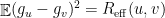
for all 


where the sum is over edges of 
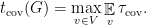
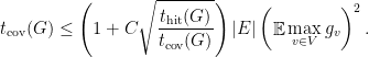
One of our main theorems can be stated as follows.
Theorem 1 (Ding-L-Peres) For every graph
where

Here 


This follows some partial progress on these questions by Kahn, Kim, Lovasz, and Vu (1999).
2. Derandomizing the cover time
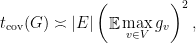
The cover time is one of the few basic graph parameters which can easily be computed by a randomized polynomial-time algorithm, but for which we don’t know of a deterministic counterpart. More precisely, for every 

We now describe one conjectural path to a better derandomization. Let 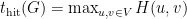

Theorem 2 There is a constant
such that for every graph
This prompts the following conjecture, which describes a potentially deeper connection between cover times and the GFF.
Conjecture 1 For a sequence of graphs
with
,
where
denotes the GFF on
.

Here, we use 


Since the proof of Theorem 1 makes heavy use of the Fernique-Talagrand majorizing measures theory for estimating 


The second part of such a derandomization strategy is the ability to compute a deterministic
Question 1 For every
, computes a
where
is a standard
-dimensional Gaussian? Is this possible if we know that
has the covariance structure of a Gaussian free field?

3. Understanding the Dynkin Isomorphism Theory
Besides majorizing measures, another major tool used in our work is the theory of isomorphisms between Markov processes and Gaussian processes. We now switch to considering the continuous-time random walk on a graph 
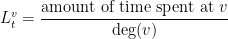
when we have run the random walk for time
Work of Ray and Knight in the 1960’s characterized the local times of Brownian motion, and then in 1980, Dynkin described a general connection between the local times of Markov processes and associated Gaussian processes. The version we use is due to Eisenbaum, Kaspi, Marcus, Rosen, and Shi (2000).
Theorem 3 Let
be given, and define the (random) time
. If
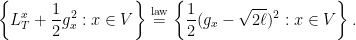
Note that on the left hand side, the local times 

Another confession we must make is that we do not really understand the actual relationship between local times… and their associated Gaussian processes. If one asks us, as is often the case during lectures, to give an intuitive description… we must answer that we cannot. We leave this extremely interesting question to you.
So I will now pass the question along. The proof of the isomorphism theorems proceeds by taking Laplace transforms and then doing some involved combinatorics. It’s analogous to the situation in enumerative combinatorics where we have a generating function proof of some equality, but not a bijective proof where you can really get your hands on what’s happening.
What is the simplest isomorphism-esque statement which has no intuitive proof? The following lemma is used in the proof of the original Ray-Knight theorem on Brownian motion (see Lemma 6.32 in the Morters-Peres book). It can be proved in a few lines using Laplace transforms, yet one suspects there should be an explicit coupling.
Lemma 4 For any
are i.i.d. standard exponentials, and
is Poisson with parameter
. If all these random variables are independent, then

Amazing! The last open question is to explain this equality of distributions in a satisfactory manner, as a first step to understanding what’s really going on in the isomorphism theory.

Those are really interesting questions!
For question 1, how much do things change if is replaced by ^2?
i.e. is it still open? still interesting?
Also, in your third equation in section 1, I think you want a 1/R_eff(u,v) in the exponent.
Hi Aram,
I think your first question didn’t come through correctly.
Also, there is no 1/R_eff(u,v) in that equation. The effective resistance comes out naturally from the fact that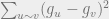 is the quadratic form arising from the Laplacian.
Aram’s first question is about a deterministic approximation to in Question 1, vs.
  . Good question.
In the regime where , by concentration properties of Gaussians, we have
so the two questions are the same. For the GFF, this corresponds to the regime in which .
.
You’re right, it may be that approximating is more natural. But it seems that for the most interesting range of parameters, the questions coincide.