As part of a summer school associated to the Hausdorff Institute for Mathematics Program on Combinatorial Optimization, I will be giving some lectures on “Semi-definite extended formulations and sums of squares.”
I wanted to post here a draft of the lecture notes. These extend and complete the series of posts here on non-negative and psd rank and lifts of polytopes. They also incorporate many corrections, and have exercises of varying levels of difficulty. The bibliographic references are sparse at the moment because I am posting them from somewhere in the Adriatic (where wifi is also sparse).
We will now prove Talagrand’s majorizing measures theorem, showing that the generic chaining bound is tight for Gaussian processes. The proof here will be a bit more long-winded than the proof from Talagrand’s book, but also (I think), a bit more accessible as well. Most importantly, we will highlight the key idea with a simple combinatorial argument.
Theorem 1 Let be a Gaussian process, and let be a sequence of subsets such that and for . Then,
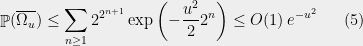
In order to make things slightly easier to work with, we look at an essentially equivalent way to state (1). Consider a Gaussian process and a sequence of increasing partitions of , where increasing means that is a refinement of for . Say that such a sequence is admissible if and for all . Also, for a partition and a point , we will use the notation for the unique set in which contains .
By choosing to be any set of points with one element in each piece of the partition , (1) yields,
We can now state our main theorem, which shows that this is essentially the only way to bound .
Theorem 2 There is a constant such that for any Gaussian process , there exists an admissible sequence which satisfies,
Theorem 3 For some constants and , the following holds. Suppose is a Gaussian process, and let be such that for . Then,
We will use only Theorem 3 and the fact that whenever to prove Theorem 2 (so, in fact, Theorem 2 holds with replaced by more general functionals satisfying an inequality like (4)).
The partitioning scheme
First, we will specify the partitioning scheme to form an admissible sequence , and then we will move on to its analysis. As discussed in earlier posts, we may assume that is finite. Every set will have a value associated with it, such that is always an upper bound on the radius of the set , i.e. there exists a point such that .
Initially, we set and . Now, we assume that we have constructed , and show how to form the partition . To do this, we will break every set into at most pieces. This will ensure that
Let be the constant from Theorem 3. Put , and let . We partition into pieces as follows. First, choose which maximizes the value
Then, set . We put .
A remark: The whole idea here is that we have chosen the “largest possible piece,” (in terms of -value), but we have done this with respect to the ball, while we cut out the ball. The reason for this will not become completely clear until the analysis, but we can offer a short explanation here. Looking at the lower bound (4), observe that the balls are disjoint under the assumptions, but we only get “credit” for the balls. When we apply this lower bound, it seems that we are throwing a lot of the space away. At some point, we will have to make sure that this thrown away part doesn’t have all the interesting stuff! The reason for our choice of vs. is essentially this: We want to guarantee that if we miss the interesting stuff at this level, then the previous level took care of it. To have this be the case, we will have to look forward (a level down), which (sort of) explains our choice of optimizing for the ball.
Now we continue in this fashion. Let be the remaining space after we have cut out pieces. For , choose to maximize the value
For , set , and put .
So far, we have been chopping the space into smaller pieces. If for some , we have finished our construction of . But maybe we have already chopped out pieces, and still some remains. In that case, we put , i.e. we throw everything else into . Since we cannot reduce our estimate on the radius, we also put .
We continue this process until is exhausted, i.e. eventually for some large enough, only contains singletons. This completes our description of the partitioning.
The tree
For the analysis, it will help to consider our partitioning process as having constructed a tree (in the most natural way). The root of the the tree is the set , and its children are the sets of , and so on. Let’s call this tree . It will help to draw and describe in a specific way. First, we will assign values to the edges of the tree. If and is a child of (i.e., and ), then the edge is given value:
If we define the value of a root-leaf path in as the sum of the edge lengths on that path, then for any ,
simply using .
Thus in order to prove Theorem 2, which states that for some ,
it will suffice to show that for some (other) constant , for any root-leaf path in , we have
Before doing this, we will fix a convention for drawing parts of . If a node has children , we will draw them from left to right. We will call an edge a right turn and every other edge will be referred to as a left turn. Note that some node may not have any right turn coming out of it (if the partitioning finished before the last step). Also, observe that along a left turn, the radius always drops by a factor of , while along a right turn, it remains the same.
We now make two observations about computing the value up to a universal constant.
Observation (1): In computing the value of a root-leaf path , we only need to consider right turns.
To see this, suppose that we have a right turn followed by a consecutive sequence of left turns. If the value of the right turn is , then the value of the following sequence of left turns is, in total, at most
In other words, because the radius decreases by a factor of along every left turn, their values decrease geometrically, making the whole sum comparable to the preceding right turn. (Recall that , so indeed the sum is geometric.)
If the problem of possibly of having no right turn in the path bothers you, note that we could artificially add an initial right turn into the root with value . This is justified since always holds. A different way of saying this is that if the path really contained no right turn, then its value is , and we can easily prove (6).
Observation (2): In computing the value of a root-leaf path , we need only consider the last right turn in any consecutive sequence of right turns.
Consider a sequence of consecutive right turns, and the fact that the radius does not decrease. The values (taking away the factor) look like . In other words, they are geometrically increasing, and thus using only the last right turn in every sequence, we only lose a constant factor.
We will abbreviate last right turn to LRT, and write to denote the value of , just counting last right turns. By the two observations, to show (6) (and hence finish the proof), it suffices to show that, for every root-leaf path in ,
The analysis
Recall that our tree has values on the edges, defined in (5). We will also put some natural values on the nodes. For a node (which, recall, is just a subset ), we put . So the edges have values and the nodes have values. Thus given any subset of nodes and edges in , we can talk about the value of the subset, which will be the sum of the values of the objects it contains. We will prove (7) by a sequence of inequalities on subsets.
Fix a root-leaf path , for which we will prove (7). Let’s prove the fundamental inequality now. We will consider two consecutive LRTs along . (If there is only one LRT in , then we are done by the preceding remarks.) See the figure below. The dashed lines represent a (possibly empty) sequence of left turns and then right turns. The two LRTs are marked.
We will prove the following inequality, which is the heart of the proof. One should understand that the inequality is on the values of the subsets marked in red. The first subset contains two nodes, and the second contains two nodes and an edge.
Figure A.
With this inequality proved, the proof is complete. Let’s see why. We start with the first LRT. Since for any node in , we have the inequality:
This gets us started. Now we apply the inequality of Figure A repeatedly to each pair of consecutive LRTs in the path . What do we have when we’ve exhausted the path ? Well, precisely all the LRTs in are marked, yielding , as desired.
The LRT inequality
Now we are left to prove the inequality in Figure A. First, let’s label some of the nodes. Let , and suppose that . The purple values are not the radii of the corresponding nodes, but they are upper bounds on the radii, recalling that along every left turn, the radius decreases by a factor of . Since there are at least two left turns in the picture, we get a upper bound on the radius of .
Part of the inequality is easy: We have since . So we can transfer the red mark from to . We are thus left to prove that
This will allow us to transfer the red mark from to the LRT coming out of and to .
When was partitioned into pieces, this was by our greedy partitioning algorithm using centers . Since we cut out the ball around each center, we have for all . Applying the Sudakov inequality (Theorem 3), we have
where the last line follows from the greedy manner in which the ‘s were chosen.
But now we claim that
This follows from two facts. First, (since actually). Secondly, the radius of is at most ! But was chosen to maximize the value of over all balls of radius , so in particular its -value is at least that of the ball containing .
Combining (9) and the preceding inequality, we prove (8), and thus that the inequality of Figure A is valid. This completes the proof.
In order to prove that the chaining argument is tight, we will need some additional properties of Gaussian processes. For the chaining upper bound, we used a series of union bounds specified by a tree structure. As a first step in producing a good lower bound, we will look at a way in which the union bound is tight.
Theorem 1 (Sudakov inequality) For some constant , the following holds. Let be a Gaussian process such that for every distinct , we have . Then,
The claim is an elementary calculation for a sequence of i.i.d. random variables (i.e. ). We will reduce the general case to this one using Slepian’s comparison lemma.
Lemma 2 (Slepian’s Lemma) Let and be two Gaussian processes such that for all ,
Then .
There is a fairly elementary proof of Slepian’s Lemma (see, e.g. the Ledoux-Talagrand book), if one is satisfied with the weaker conclusion , which suffices for our purposes.
To see that Lemma 2 yields Theorem 1, take a family with for all and consider the associated variables where is a family of i.i.d. random variables. It is straightforward to verify that (1) holds, hence by the lemma, , and the result follows from the i.i.d. case.
The Sudakov inequality gives us “one level” of a lower bound; the following strengthening will allow us to use it recursively. If we have a Gaussian process and , we will use the notation
For and , we also use the notation
Here is the main theorem of this post; its statement is all we will require for our proof of the majorizing measures theorem:
Theorem 3 For some constants and , the following holds. Suppose is a Gaussian process, and let be such that for . Then,
The proof of the preceding theorem relies on the a strong concentration property for Gaussian processes. First, we recall the classical isoperimetric inequality for Gaussian space (see, for instance, (2.9) here).
We remind the reader that for a function ,
Theorem 4 Let , and let , where is the standard -dimensional Gaussian measure. Then,
Using this, we can prove the following remarkable fact.
Theorem 5 Let be a Gaussian process, then
A notable aspect of this statement is that only the maximum variance affects the concentration, not the number of random variables. We now prove Theorem 5 using Theorem 4.
Proof: We will prove it in the case , but of course our bound is independent of . The idea is that given a Gaussian process , we can write
for , where are standard i.i.d. normals, and the matrix is a matrix of real coefficients. In this case, if is a standard -dimensional Gaussian, then the vector is distributed as .
If we put , then Theorem 4 yields (3) as long as . It is easy to see that
But is just the maximum norm of any row of , and the norm of row is
Using this theorem, we are ready to prove Theorem 3. I will only give a sketch here, but filling in the details is not too difficult.
Assume that the conditions of Theorem 3 hold. Pick an arbitrary , and recall that we can write
so we could hope that for some , we simultaneously have , yielding
The problem, of course, is that the events we are discussing are not independent.
This is where Theorem 5 comes in. For any , all the variances of the variables are bounded by . This implies that we can choose a constant such that
So, in fact, we can expect that none of the random variables will deviate from its expected value by more than . Which means we can (morally) replace (4) by
When it is impossible to achieve a low-distortion embedding of some space into another space , we can consider more lenient kinds of mappings which are still suitable for many applications. For example, consider the unweighted -cycle . It is known that any embedding of into a tree metric incurs distortion . On the other hand, if we delete a uniformly random edge of , this leaves us with a random tree (actually a path) such that for any , we have
In other words, in expectation the distortion is only 2.
Let be a finite metric space, and let be a family of finite metric spaces. A stochastic embedding from into is a random pair where and is a non-contractive mapping, i.e. such that for all . The distortion of is defined by
Theorem 1 Every -point metric space admits a stochastic embedding into the family of tree metrics, with distortion .
We will need the random partitioning theorem we proved last time:
Theorem 2 For every , there is a -bounded random partition of which satisfies, for every and ,
From partitions to trees. Before proving the theorem, we discuss a general way of constructing a tree metric from a sequence of partitions. Assume (by perhaps scaling the metric first) that for all with . Let be partitions of , where is -bounded. We will assume that and is a partition of into singleton sets.
Now we inductively construct a tree metric as follows. The nodes of the tree will be of the form for and . The root is . In general, if the tree has a node of the form for , then will have children
The length of an edge of the form is . This specifies the entire tree . We also specify a map by . We leave the following claim to the reader.
Claim 1 For every ,
where is the largest index with .
Note, in particular, that is non-contracting because if for some , then since is -bounded, implying that .
Proof: Again, assume that for all . For , let be the -bounded random partition guaranteed by Theorem 2. Let be a partition into singletons, and let . Finally, let be the tree constructed above, and let be the corresponding (random) non-contractive mapping.
Now, fix and an integer such that . Using Claim 1 and (1), we have,
where in the penultimate line, we have evaluated three disjoint telescoping sums: For any numbers ,
Since every tree embeds isometrically into , this offers an alternate proof of Bourgain’s theorem when the target space is . Since we know that expander graphs require distortion into , this also shows that Theorem 1 is asymptotically tight.
In addition to the current sequence on Talagrand’s majorizing measures theory, I’m also going to be putting up a series of lecture notes about embeddings of finite metric spaces. The first few will concern random partitions of metric spaces, and their many applications.
Random partitions
Often when one is confronted with the problem of analyzing some problem on a metric space , a natural way to proceed is by divide and conquer: Break the space into small pieces, do something (perhaps recursively) on each piece, and then glue these local solutions together to achieve a global result. This is certainly an important theme in areas like differential geometry, harmonic analysis, and computational geometry.
In the metric setting, “small” often means pieces of small diameter. Of course we could just break the space into singletons , but this ignores the second important aspect in a “divide and conquer” approach: what goes on at the boundary. If we are going to combine our local solutions together effectively, we want the “boundary” between distinct pieces of the partition to be small. Formalizing this idea in various ways leads to a number of interesting ideas which I’ll explore in a sequence of posts.
Example: The unit square
Consider the unit square in the plane, equipped with the metric. If we break the square into pieces of side length , then every piece has diameter at most , and a good fraction of the space is far from the boundary of the partition. In fact, it is easy to see that e.g. 60% of the measure is at least distance from the boundary (the red dotted line).
But there is a problem with using this as a motivating example. First, observe that we had both a metric structure (the distance) and a measure (in this case, the uniform measure on ). In many potential applications, there is not necessarily a natural measure to work with (e.g. for finite metric spaces, where counting the number of points is often a poor way of measuring the “size” of various pieces).
To escape this apparent conundrum, note that the uniform measure is really just a distraction: The same result holds for any measure on . This is a simple application of the probabilistic method: If we uniformly shift the -grid at random, then for any point , we have
Thus, by averaging, for any measure on there exists a partition where 60% of the -measure is -far from the boundary. This leads us to the idea that, in many situations, instead of talking about measures, it is better to talk about distributions over partitions. In this case, we want the “boundary” to be small on “average.”
Lipschitz random partitions
We will work primarily with finite metric spaces to avoid having to deal with continuous probability spaces; much of the theory carries over to general metric spaces without significant effort (but the development becomes less clean, as this requires certain measurability assumptions in the theorem statements).
Let be a finite metric space. If is a partition of , and , we will write for the unique set in containing . We say that is -bounded if for all . We will also say that a random partition is -bounded if it is supported only on -bounded partitions of .
Let’s now look at one way to formalize the idea that the “boundary” of a random partition is small.
A random partition of is -Lipschitz if, for every ,
Intuitively, the boundary is small if nearby points tend to end up in the same piece of the partition. There is a tradeoff between a random partition being -bounded and -Lipschitz. As increases, we expect that we can make , and hence the “boundary effect,” smaller and smaller. The following theorem can be derived from work of Leighton and Rao, or Linial and Saks. The form stated below comes from work of Bartal.
Theorem 1
If is an -point metric space and , then for every , there is an -Lipschitz, -bounded random partition of .
We will prove a more general fact that will be essential later. For positive numbers , define (note that ). The next theorem and proof are from Calinescu, Karloff, and Rabani.
Theorem 2
For every , there is a -bounded random partition of which satisfies, for every and ,
Observe that Theorem 1 follows from Theorem 2 by setting , and noting that implies . We also use for .
Proof:
Suppose that . Let be chosen uniformly at random, and let be a uniformly random bijection . We will think of as giving a random ordering of . We define our random partition as follows.
For , define
It is straightforward that is a partition of , with perhaps many of the sets being empty. Furthermore, by construction, is -bounded. Thus we are left to verify (1).
To this end, fix and , and enumerate the points of so that . Let . We will say that a point sees if , and we will say that cuts if .
(In the picture below, and see , while does not. Only cuts .)
Observe that for any ,
Using this language, we can now reveal our analysis strategy: Let be the minimal element (according to the ordering ) which sees . Then can only occur if also cuts . The point is that the fate of is not decided until some point sees . Then, if does not cut , we have , hence .
Thus we can write,
To analyze the latter sum, first note that if , then can never see since always. On the other hand, if then always sees , but can never cut since always.
Recalling that by assumption, and setting and let , we can use (3) to write
Now we come to the heart of the analysis: For any ,
The idea is that if cuts , then . Thus if any for comes before in the -ordering, then also sees since , hence . But the probability that is the -minimal element of is precisely , proving (5).
To finish the proof, we combine (2), (4), and (5), yielding
Tightness for expanders. Before ending this section, let us mention that Theorem 1 is optimal up to a constant factor. Let be a family of degree-3 expander graphs, equipped with their shortest-path metric . Assume that for some and all . Let , and suppose that admits a -bounded -Lipschitz random partition. By averaging, this means there is a fixed -bounded partition of which cuts at most an -fraction of edges. But every has , which implies . Hence the partition must cut an fraction of edges, implying .
In the next post, we’ll see how these random partitions allow us to reduce may questions on finite metric spaces to questions on trees.
In the last post, we considered a Gaussian process and were trying to find upper bounds on the quantity . We saw that one could hope to improve over the union bound by clustering the points and then taking mini union bounds in each cluster.
Hierarchical clustering
To specify a clustering, we’ll take a sequence of progressively finer approximations to our set . First, recall that we fixed , and we have used the observation that .
Now, assume that is finite. Write , and consider a sequence of subsets such that . We will assume that for some large enough , we have for . For every , let denote a “closest point map” which sends to the closest point in .
The main point is that we can now write, for any ,
This decomposition is where the term “chaining” arises, and now the idea is to bound the probability that is large in terms of the segments in the chain.
What should look like?
One question that arises is how we should think about choosing the approximations . We are trading off two measures of quality: The denser is in the set (or, more precisely, in the set ) the smaller the variances of the segments will be. On the other hand, the larger is, the more segments we’ll have to take a union bound over.
So far, we haven’t used any property of our random variables except for the fact that they are centered. To make a more informed decision about how to choose the sets , let’s recall the classical Gaussian concentration bound.
Lemma 1 For every and ,
This should look familiar: is a mean-zero Gaussian with variance .
Now, a first instinct might be to choose the sets to be progressively denser in . In this case, a natural choice would be to insist on something like being a -net in . If one continues down this path in the right way, a similar theory would develop. We’re going to take a different route and consider the other side of the tradeoff.
Instead of insisting that has a certain level of accuracy, we’ll insist that is at most a certain size. Should we require or , or use some other function? To figure out the right bound, we look at (2). Suppose that are i.i.d. random variables. In that case, applying (2) and a union bound, we see that to achieve
we need to select . If we look instead at points instead of points, the bound grows to . Thus we can generally square the number of points before the union bound has to pay a constant factor increase. This suggests that the right scaling is something like . So we’ll require that for all .
The generic chaining
This leads us to the generic chaining bound, due to Fernique (though the formulation we state here is from Talagrand).
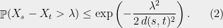
Theorem 2 Let be a Gaussian process, and let be a sequence of subsets such that and for . Then,
Proof: As before, let denote the closest point map and let . Using (2), for any , , and , we have
Now, the number of pairs can be bounded by , so we have
Theorem 1.2 gives us a fairly natural way to upper bound the expected supremum using a hierarchical clustering of . Rather amazingly, as we’ll see in the next post, this upper bound is tight. Talagrand’s majorizing measure theorem states that if we take the best choice of in Theorem 1.2, then the upper bound in (3) is within a constant factor of .
It’s most intuitive to start with the geometric viewpoint, in which case an -simplex is defined to be the convex hull of affinely independent points in . These points are called the vertices of the simplex. Here are examples for
A simplicial complexis then a collection of simplices glued together along lower-dimensional simplices. More formally, if is a (geometric) simplex, then a face of is a subset formed by taking the convex hull of a subset of the vertices of .
Finally, a (geometric) simplicial complex is a collection of simplices such that
If and is a face of , then , and
If and , then is a face of both and .
Property (1) gives us downward closure, and property (2) specifies how simplices can be glued together (only along faces). For instance, the first picture depicts a simplicial complex. The second does not.
Continuing our look at some toplogical methods, today we’ll see the evasiveness conjecture in decision tree complexity. In the next lecture, we’ll see how we can sometimes analyze the complexity using fixed point theorems, and their generalizations (like the Hopf index formula), following the work of Kahn, Saks, and Sturtevant. These two lectures are co-blogged with Elisa Celis, with a lot of input from Lovasz’s lecture notes.
Decision tree complexity and evasiveness
Consider a boolean function on n bits. We define the decision tree complexity of f as follows. Given an unknown input , you are allowed to ask about the values of various bits of x, e.g. . Your goal is to compute using as few questions as possible, and your questions can be adaptive, depending on answers to previous questions. The complexity of such a strategy is the maximum number of questions asked for any . The decision tree complexity, written , is the minimum complexity of any strategy that computes f. (There are many other interesting models of decision complexity, see e.g. this survey.)
Clearly , because we can trivially query all the bits of x, and then output f(x). A function f is called evasive if this upper bound is met, i.e. . As an example, consider the parity function , where is addition modulo 2. Clearly is evasive because after bits of x are asked about, the setting of the final bit determines the value of f.
For a more general example, consider any such that is odd. In this case, for every , exactly one of or has the same property that the number of inputs resulting in a 1 is odd. (These two functions are the natural restriction of f to functions on n-1 bits, which results from fixing the value of the ith bit.) Thus an adversary could keep answering questions “?” so that the restricted function retains this property. Since the number of inputs yielding a 1 is always odd, the restricted function always takes both possible values, implying that f is evasive–the advesary ensures that the value cannot be determined until all n possible questions are asked.
For an example of a non-evasive property, think of a point as speciying a directed graph on vertices, where there is exactly one directed edges connecting every pair of vertices, and x specifies the direction of this edge (this is called a tournament). Thinking of the vertices as players, a directed edge from u to v means that u defeats v. Now if the digraph specified by x has one vertex that defeats everyone else. What is ?
Well, first we can conduct a single elimination tournament, where vertex 1 plays vertex 2, and the winner players vertex 3, and the winner of that players vertex 4, etc. At the end, there is only one remaining vertex that remains undefeated. Now asking more questions, we can determine whether indeeds defeats everyone else. The total number of questions was , hence , implying that f is not evasive.
Montone graph properties and the evasiveness conjecture
Let . In general, we can encode an arbitrary undirected N-vertex graph as an element . A function is called a graph property if relabeling the vertices of doesn’t affect the value of . The function f is monotone if the value of the function can never change from 1 to 0 when flipping one of the input bits from 0 to 1. In the setting of graph properties, this corresponds to those which are maintained under addition of edges to the graph, e.g. “is G connected?” or “does G have a k-clique?”
Evasiveness Conjecture (Aanderaa-Karp-Rosenberg): Every non-trivial monotone graph property is evasive.
Here, non-trivial means that , where and denote the all-zeros and all-ones strings, respectively.
For example, consider the example “is G connected?” The adversary is simple: When asked about a possible edge , she answers NO unless this answer would imply that the graph is disconnected. In other words, she answers NO unless she has answered NO already for all edges across a cut except for , in which case she has to answer YES.
Now, suppose there is a strategy which figures out the connectivity of without asking a question about some edge . In this case, the conclusion must be that because the adversary always maintains that by answering everything in the future YES, she could force the graph to be connected. In this case, the edges answered YES have to form a spanning tree of G (otherwise by answering all unasked questions NO, the graph would become disconnected). Consider a path P from i to j in this YES spanning tree. Let be the edge of P which was asked about last. Clearly the adversary answered YES for , but this contradicts the advesary’s strategy. Since has not been asked yet, the adversary is safe to answer NO for , and still later by answering YES on , she could force the graph to be connected. Thus no such strategy exists, and connectivity is evasive.
Now we’ll move away from spectral methods, and into a few lectures on topological methods. Today we’ll look at the Borsuk-Ulam theorem, and see a stunning application to combinatorics, given by Lovász in the late 70’s. A great reference for this material is Matousek’s book, from which I borrow heavily. I’ll also discuss why the Lovász-Kneser theorem arises in theoretical CS.
The Borsuk-Ulam Theorem
We begin with a statement of the theorem. We will think of the n-dimensional sphere as the subset of given by
Borsuk-Ulam Theorem: For every continuous mapping , there exists a point with .
Pairs of points are called antipodal.
There are a couple of common illustrative examples for the case . The theorem says that if you take the air out of a basketball, crumple it (no tearing), and flatten it out, then there are two points directly on top of each other which were antipodal before. Another common example states that at every point in time, there must be two points on the earth which both have exactly the same temperature and barometric pressure (assuming, of course, that these two parameters vary continuously over the surface of the eath).
The n=1 case is completely elementary. For the rest of the lecture, let’s use and to denote the north and south poles (the dimension will be obvious from context). To prove the n=1 case, simply trace out the path in starting at and going clockwise around . Simultaneously, trace out the path starting at and going counter-clockwise at the same speed. It is easy to see that eventually these two paths have to collide: At the point of collision, .
We will give the sketch of a proof for Let , and note that our goal is to prove that for some . Note that is antipodal in the sense that for all . Now, if for every , then by compactness there exists an such that for all . Because of this, we may approximate arbitrarily well by a smooth map, and prove that the approximation has a 0. So we will assume that itself is smooth.
Now, define by , i.e. the north/south projection map. Let be a hollow cylinder, and let be given by so that linearly interpolates between and .
Also, let’s define an antipodality on by . Note that is antipodal with respect to , i.e. , because both and are antipodal. For the sake of contradiction, assume that for all .
Now let’s consider the structure of the zero set . Certainly since , and these are h’s only zeros. Here comes the sketchy part: Since is smooth, is also smooth, and thus locally can be approximated by an affine mapping . It follows that if is not empty, then it should be a subspace of dimension at least one. By an arbitrarily small perturbation of the initial , ensuring that is sufficiently generic, we can ensure that is either empty or a subspace of dimension one. Thus locally, should look like a two-sided curve, except at the boundaries and , where (if non-empty) would look like a one-sided curve. But, for instance, cannot contain any Y-shaped branches.
It follows that is a union of closed cycles and paths whose endpoints must lie at the boundaries and . ( is represented by red lines in the cylinder above.) But since there are only two zeros on the sphere, and none on the sphere, must contain a path from to Since is antipodal with respect to , must also satisfy this symmetry, making it impossible for the segment initiating at N to ever meet up with the segment initiating at S. Thus we arrive at a contradiction, implying that must take the value 0.
Notice that the only important property we used about (other than its smoothness) is that is has a number of zeros which is twice an odd number. If had, e.g. four zeros, then we could have two -symmetric paths emanating from and returning to the bottom. But if has six zeros, then we would again reach a contradiction.
In the previous lecture, we gave an upper bound on the second eigenvalue of the Laplacian of (bounded degree) planar graphs in order to analyze a simple spectral partitioning algorithm. A natural question is whether these bounds extend to more general families of graphs. Well-known generalizations of planar graphs are those which can be embedded on a surface of fixed genus, and, more generally, families of graphs that arise by forbidding minors. In fact, Spielman and Teng conjectured that for any graph excluding as a minor, one should have . Of course planar graphs have genus 0, and by Wagner’s theorem, are precisely the graphs which exclude and as minors. In this lecture, we will follow an intrinsic approach of Biswal, myself, and Rao which, in particular, is able to resolve the conjecture of Spielman and Teng. First, we see why even pushing the conformal approach to bounded genus graphs is difficult.
Bounded genus graphs
For graphs of bounded genus, there is hope to use an approach based on conformal mappings. In 1980, Yang and Yau proved that
for any compact Riemannian surface of genus . (Note that for the Laplace-Beltrami operator, one usually writes as the first non-zero eigenvalue, rather than .) In analog with Hersch’s proof of the genus 0 case, they use Riemann-Roch to obtain a degree- conformal mapping to the Riemann sphere, then try to pull back a second eigenfunction. A factor of the degree is lost in the Rayleigh quotient (hence the factor in the preceding bound), and Hersch’s Möbius trick is still required.
genus 0
genus 1
genus 2
genus 3
An analogous proof for graphs of bounded genus would proceed by constructing a circle packing of on the sphere , but instead of the circles having disjoint interiors, we would be assured that every point of is contained in at most circles. Unfortunately, such a result is impossible (this has to do with the handling of branch points in the discrete setting). Kelner has to take a different approach in his proof that for graphs of genus at most .
He starts with a circle packing of on a compact surface of genus (whose existence follows from results of Beardon and Stephenon and He and Schramm). Then Kelner randomly subdivides repeatedly, and these subdivisions give progressively better approximations to some sequence of surfaces . Once the approximation is of high enough quality, one applies Riemann-Roch to , and infers something about a subdivision of . The final element is to track how the second eigenvalue of changes (in expectation) under random subdivision.
Needless to say, this approach is already quite delicate, and for graphs that can’t be equipped with some kind of conformal structure, we seem to have reached a dead end. In this lecture, we’ll see how to use intrinsic deformations of the geometry of in order to bound its eigenvalues. Eventually, this will reduce to the study of certain kinds of multi-commodity flows.
Metrics on graphs
Let be an arbitrary n-vertex graph with maximum degree . Recall that we can write
where . (Also recall that we can replace by any Hilbert space, and the same formula holds.) The first step is to prepare this equality for “non-linearization” by getting rid of the linear condition and the sum . (This is a popular sort of passage in the non-linear geometry of Banach spaces, which also plays a rather important role in applications to the theoretical CS.) The goal is to get only terms that look like . Fortunately, there is a well-known way to do this:
which follows easily from the equality when .
Thus if we want to bound , we need to find an for which the latter ratio (without the ) is . Now, for someone who works a lot with linear programming relaxations, it’s very natural to consider a “relaxation”
where the minimization is over all pseudo-metrics d, i.e. symmetric non-negative functions which satisfy the triangle inequality, but might have even for . Certainly , but Bourgain’s embedding theorem (which states that every n-point metric space embeds into a Hilbert space with distortion at most ) also assures us that . Since we are trying to show that , this term is morally negligible. One can see the paper for a more advanced embedding argument that doesn’t lose this factor, but for now we concentrate on proving that . The embedding theorems allow us to concentrate on finding an intrinsic metric on the graph with small “Rayleigh quotient,” without having to worry about an eventual geometric representation.
As a brief preview… we are going to find a good metric by taking a certain kind of all-pairs multi-commodity flow at optimality, and weighting the edges by their congestion in the optimal flow. Thus as the flow spreads out on the graph, it has the effect of “uniformizing” its geometry.
Discrete Riemannian metrics, convexification, and duality
Let’s now assume that is planar. We want to show that . First, let’s restrict ourselves to vertex weighted metrics on . Given any non-negative weight function , we can define the length of a path in by summing the weights of vertices along it: . Then we can define a vertex-weighted shortest-path pseudo-metric on in the natural way
where is the set of all u-v paths in . We also have the nice relationship
since .
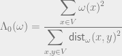
So if we define
then by (1), we have .
Examples. Let’s try to exhibit weights for two well-known examples: the grid, and the complete binary tree.
For the grid, we can simply take for all . Clearly . On the other hand, a random pair of points in the grid is apart, hence . It follows that , as desired.
For the complete binary tree with root , we can simply put and for . (Astute readers will guess the geometrically decreasing weights are actually the optimal choice.) In this case, , while all the pairs on opposite sides of the root have . It again follows that . Our goal is to provide such a weight for any planar graph.
 be a Gaussian process, and let
  be a sequence of subsets such that
  and
and  for
for  . Then,
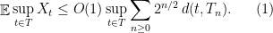
 of
of  , where increasing means that
  is a refinement of
  for
for  . Say that such a sequence
  is admissible if
  and
and  for all
  and a point
  , we will use the notation
  for the unique set in
  .
. to be any set of points with one element in each piece of the partition
 .
. such that for any Gaussian process
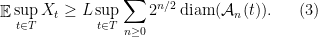
 , we defined
 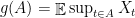 , and in the last post,
  and
and  , the following holds. Suppose
  be such that
  for
for  . Then,
 whenever
  to prove Theorem
  will have a value
  associated with it, such that
  , i.e. there exists a point
  such that
  .
. . Now, we assume that we have constructed
  pieces. This will ensure that
 be the constant from Theorem
  , and let
  . We partition
  pieces as follows. First, choose
  which maximizes the value
 . We put
  .
. -value), but we have done this with respect to the
  ball, while we cut out the
  ball. The reason for this will not become completely clear until the analysis, but we can offer a short explanation here. Looking at the lower bound
  are disjoint under the assumptions, but we only get “credit” for the
  balls. When we apply this lower bound, it seems that we are throwing a lot of the space away. At some point, we will have to make sure that this thrown away part doesn’t have all the interesting stuff! The reason for our choice of
  be the remaining space after we have cut out
  pieces. For
  , choose
  to maximize the value
 , set
, set  , and put
  .
. for some
  pieces, and still some remains. In that case, we put
  , i.e. we throw everything else into
  . Since we cannot reduce our estimate on the radius, we also put
  .
. large enough,
  , and so on. Let’s call this tree
  . It will help to draw and describe
  is a child of
  and
and  ), then the edge
  is given value:
 and
and 
 .
.

 , we will draw them from left to right. We will call an edge
  a right turn and every other edge will be referred to as a left turn. Note that some node
 up to a universal constant.
 , then the value of the following sequence of left turns is, in total, at most
 . This is justified since
  always holds. A different way of saying this is that if the path really contained no right turn, then its value is
  , and we can easily prove
  factor) look like
  . In other words, they are geometrically increasing, and thus using only the last right turn in every sequence, we only lose a constant factor.
 to denote the value of
 ), we put
  . So the edges have values and the nodes have values. Thus given any subset of nodes and edges in

 for any node
  in
in  , we have the inequality:
 ? Well, precisely all the LRTs in
  , as desired.
 .
.
 since
since  . So we can transfer the red mark from
  to
to  . We are thus left to prove that
 . Since we cut out the
  for all
 ‘s were chosen.
 (since
  actually). Secondly, the radius of
  was chosen to maximize the value of
  over all balls of radius
  , the following holds. Let
  be a Gaussian process such that for every distinct
  , we have
  . Then,
 random variables
  (i.e.
(i.e.  ). We will reduce the general case to this one using Slepian’s comparison lemma.
 be two Gaussian processes such that for all
 .
.  , which suffices for our purposes.
 and consider the associated variables
  where
where  is a family of i.i.d.
  , and the result follows from the i.i.d. case.
 , we will use the notation
 and
and  , we also use the notation
 and
and  , the following holds. Suppose
  be such that
  for
for  . Then,

 ,
,
 , where
  is the standard
  -dimensional Gaussian measure. Then,

 , but of course our bound is independent of
  , we can write
 , where
  are standard i.i.d. normals, and the matrix
  is a matrix of real coefficients. In this case, if
  is a standard
  is distributed as
  .
. , then Theorem
  . It is easy to see that
 is just the maximum
  norm of any row of
  , and the
  is
is 


 , and recall that we can write

 achieves this. By definition,
 , we simultaneously have
  , yielding
 are bounded by
  . This implies that we can choose a constant
  such that
 random variables
  will deviate from its expected value by more than
  . Which means we can (morally) replace
 , the error term is absorbed.
  into another space
  , we can consider more lenient kinds of mappings which are still suitable for many applications. For example, consider the unweighted
  . It is known that any embedding of
  . On the other hand, if we delete a uniformly random edge of
  such that for any
  , we have
 ![\displaystyle d_{C'_n}(x,y) \geq d_{C_n}(x,y) \geq \frac12\, \mathop{\mathbb E}[d_{C'_n}(x,y)].](https://s0.wp.com/latex.php?latex=%5Cdisplaystyle++d_%7BC%27_n%7D%28x%2Cy%29+%5Cgeq+d_%7BC_n%7D%28x%2Cy%29+%5Cgeq+%5Cfrac12%5C%2C+%5Cmathop%7B%5Cmathbb+E%7D%5Bd_%7BC%27_n%7D%28x%2Cy%29%5D.+&bg=eeeeee&fg=000000&s=0&c=20201002)
 be a finite metric space, and let
  be a family of finite metric spaces. A stochastic embedding from
  where
where  and
and  is a non-contractive mapping, i.e. such that
  for all
  . The distortion of
  is defined by
 ![\displaystyle \max_{x,y \in X} \frac{\mathop{\mathbb E} \left[d_Y(F(x),F(y))\right]}{d_X(x,y)}\,.](https://s0.wp.com/latex.php?latex=%5Cdisplaystyle++%5Cmax_%7Bx%2Cy+%5Cin+X%7D+%5Cfrac%7B%5Cmathop%7B%5Cmathbb+E%7D+%5Cleft%5Bd_Y%28F%28x%29%2CF%28y%29%29%5Cright%5D%7D%7Bd_X%28x%2Cy%29%7D%5C%2C.+&bg=eeeeee&fg=000000&s=0&c=20201002)
 .
.  , there is a
  -bounded random partition
  of
of  and
and  ,
, 
 for all
  . Let
. Let  be partitions of
  is
is  -bounded. We will assume that
  and
and  is a partition of
 as follows. The nodes of the tree will be of the form
  for
for  and
and  . The root is
  . In general, if the tree has a node of the form
  for
for  , then
 is
is  . This specifies the entire tree
  . We also specify a map
  by
by  . We leave the following claim to the reader.
 is the largest index with
  .
.  for some
  , then
  is
is  .
. , let
, let  be the
  be a partition into singletons, and let
  . Finally, let
  be the tree constructed above, and let
  be the corresponding (random) non-contractive mapping.
 such that
  . Using Claim
 ![\displaystyle \mathop{\mathbb E}\left[d_{\mathcal T}(F(x),F(y))\right] \leq \sum_{j=0}^M \mathop{\mathbb P}[\mathcal P_j(x) \neq \mathcal P_j(y)] \cdot 2^{j+3}](https://s0.wp.com/latex.php?latex=%5Cdisplaystyle++%5Cmathop%7B%5Cmathbb+E%7D%5Cleft%5Bd_%7B%5Cmathcal+T%7D%28F%28x%29%2CF%28y%29%29%5Cright%5D+%5Cleq+%5Csum_%7Bj%3D0%7D%5EM+%5Cmathop%7B%5Cmathbb+P%7D%5B%5Cmathcal+P_j%28x%29+%5Cneq+%5Cmathcal+P_j%28y%29%5D+%5Ccdot+2%5E%7Bj%2B3%7D++&bg=eeeeee&fg=000000&s=0&c=20201002)


 ,
, 
 , this offers an alternate proof of Bourgain’s theorem when the target space is
  distortion into
  , this also shows that Theorem
  , but this ignores the second important aspect in a “divide and conquer” approach: what goes on at the boundary. If we are going to combine our local solutions together effectively, we want the “boundary” between distinct pieces of the partition to be small. Formalizing this idea in various ways leads to a number of interesting ideas which I’ll explore in a sequence of posts.
![{[0,1]^2}](https://s0.wp.com/latex.php?latex=%7B%5B0%2C1%5D%5E2%7D&bg=eeeeee&fg=000000&s=0&c=20201002) in the plane, equipped with the
in the plane, equipped with the  , then every piece has diameter at most
  , and a good fraction of the space is far from the boundary of the partition. In fact, it is easy to see that e.g. 60% of the measure is at least distance
  from the boundary (the red dotted line).
 2
2![{x \in [0,1]^2}](https://s0.wp.com/latex.php?latex=%7Bx+%5Cin+%5B0%2C1%5D%5E2%7D&bg=eeeeee&fg=000000&s=0&c=20201002) , we have
, we have
 on
on  is a partition of
  for the unique set in
  . We say that
  for all
  . We will also say that a random partition
  -bounded if it is supported only on
  -Lipschitz if, for every
 , then for every
  -Lipschitz,
  , define
  (note that
  ). The next theorem and proof are from
 , and noting that
  implies
  . We also use
  for
for  . Let
. Let ![{\alpha \in [\frac14, \frac12]}](https://s0.wp.com/latex.php?latex=%7B%5Calpha+%5Cin+%5B%5Cfrac14%2C+%5Cfrac12%5D%7D&bg=eeeeee&fg=000000&s=0&c=20201002) be chosen uniformly at random, and let
be chosen uniformly at random, and let  be a uniformly random bijection
  . We will think of
  , define
 is a partition of
  , with perhaps many of the sets
  being empty. Furthermore, by construction,
  , and enumerate the points of
  so that
  . Let
. Let  . We will say that a point
  sees
sees  if
if  , and we will say that
  .
. and
and  see
see  , while
  does not. Only
 ,
,![\displaystyle \mathbb P\left(y \textrm{ cuts } B\right) = \mathbb P\left(\alpha \Delta \in [d(x,y)-r,d(x,y)+r]\right) \leq \frac{2r}{\Delta/4} = \frac{8r}{\Delta}.\ \ \ \ \ (2)](https://s0.wp.com/latex.php?latex=%5Cdisplaystyle+%5Cmathbb+P%5Cleft%28y+%5Ctextrm%7B+cuts+%7D+B%5Cright%29+%3D+%5Cmathbb+P%5Cleft%28%5Calpha+%5CDelta+%5Cin+%5Bd%28x%2Cy%29-r%2Cd%28x%2Cy%29%2Br%5D%5Cright%29+%5Cleq+%5Cfrac%7B2r%7D%7B%5CDelta%2F4%7D+%3D+%5Cfrac%7B8r%7D%7B%5CDelta%7D.%5C+%5C+%5C+%5C+%5C+%282%29&bg=eeeeee&fg=000000&s=0&c=20201002)
 be the minimal element (according to the ordering
  is not decided until some point sees
  , hence
  .
.
 , then
  can never see
  always. On the other hand, if
  then
then  always.
 by assumption, and setting
  and let
  , we can use
 . Thus if any
  for
for  comes before
  , hence
  . But the probability that
  is precisely
  , proving
 be a family of degree-3 expander graphs, equipped with their shortest-path metric
  . Assume that
  for some
  and all
  . Let
. Let  , and suppose that
  admits a
  -bounded
  , which implies
  . Hence the partition must cut an
  fraction of edges, implying
  .
. . We saw that one could hope to improve over the union bound by clustering the points and then taking mini union bounds in each cluster.
 .
. , and consider a sequence of subsets
  such that
  . We will assume that for some large enough
  for
for  . For every
  , let
, let  denote a “closest point map” which sends
  to the closest point in
  .
.
 is large in terms of the segments in the chain.
 look like?
  ) the smaller the variances of the segments
  will be. On the other hand, the larger
  ,
, 
 is a mean-zero Gaussian with variance
  .
. -net in
  or
or  , or use some other function? To figure out the right bound, we look at
  are i.i.d.
 . If we look instead at
  points instead of
  . Thus we can generally square the number of points before the union bound has to pay a constant factor increase. This suggests that the right scaling is something like
  . So we’ll require that
  for all
  .
. be a sequence of subsets such that
  and
and  for
for 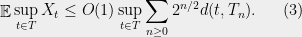
 , we have
 can be bounded by
  , so we have

 , since we get geometrically decreasing summands.
 occurs, then
  . Thus
  ,
, 


 .
. -simplex is defined to be the convex hull of
 . These points are called the vertices of the simplex. Here are examples for


 is a (geometric) simplex, then a face of
  is a subset
  formed by taking the convex hull of a subset of the vertices of
  of simplices such that
 and
and  is a face of
  , and
, and and
and  , then
  is a face of both
  .
.

 on n bits. We define the decision tree complexity of f as follows. Given an unknown input
  , you are allowed to ask about the values of various bits of x, e.g.
  . Your goal is to compute
  using as few questions as possible, and your questions can be adaptive, depending on answers to previous questions. The complexity of such a strategy is the maximum number of questions asked for any
  , is the minimum complexity of any strategy that computes f. (There are many other interesting models of decision complexity, see e.g.
 , because we can trivially query all the bits of x, and then output f(x). A function f is called evasive if this upper bound is met, i.e.
  . As an example, consider the parity function
  , where
  is addition modulo 2. Clearly
  is evasive because after
  bits of x are asked about, the setting of the final bit determines the value of f.
 is odd. In this case, for every
  , exactly one of
  or
or  has the same property that the number of inputs resulting in a 1 is odd. (These two functions are the natural restriction of f to functions on n-1 bits, which results from fixing the value of the ith bit.) Thus an adversary could keep answering questions “
 ?” so that the restricted function retains this property. Since the number of inputs yielding a 1 is always odd, the restricted function always takes both possible values, implying that f is evasive–the advesary ensures that the value cannot be determined until all n possible questions are asked.
 as speciying a directed graph on
  vertices, where there is exactly one directed edges connecting every pair of vertices, and x specifies the direction of this edge (this is called a
  if the digraph specified by x has one vertex that defeats everyone else. What is
  that remains undefeated. Now asking
  more questions, we can determine whether
  , hence
  , implying that f is not evasive.
 . In general, we can encode an arbitrary undirected N-vertex graph as an element
  . A function
  is called a graph property if relabeling the vertices of
  doesn’t affect the value of
  . The function f is monotone if the value of the function can never change from 1 to 0 when flipping one of the input bits from 0 to 1. In the setting of graph properties, this corresponds to those which are maintained under addition of edges to the graph, e.g.
  “is G connected?” or
  “does G have a k-clique?”
 , where
  and
and  denote the all-zeros and all-ones strings, respectively.
 , she answers NO unless this answer would imply that the graph is disconnected. In other words, she answers NO unless she has answered NO already for all edges across a cut
  except for
  because the adversary always maintains that by answering everything in the future YES, she could force the graph to be connected. In this case, the edges answered YES have to form a spanning tree of G (otherwise by answering all unasked questions NO, the graph would become disconnected). Consider a path P from i to j in this YES spanning tree. Let
  be the edge of P which was asked about last. Clearly the adversary answered YES for
 given by
 , there exists a point
  with
with  .
. are called antipodal.
 . The theorem says that if you take the air out of a basketball, crumple it (no tearing), and flatten it out, then there are two points directly on top of each other which were antipodal before. Another common example states that at every point in time, there must be two points on the earth which both have exactly the same temperature and barometric pressure (assuming, of course, that these two parameters vary continuously over the surface of the eath).
 and
and  to denote the north and south poles (the dimension will be obvious from context). To prove the n=1 case, simply trace out the path in
  starting at
  and going clockwise around
  . Simultaneously, trace out the path starting at
  and going counter-clockwise at the same speed. It is easy to see that eventually these two paths have to collide: At the point of collision,
  Let
Let  , and note that our goal is to prove that
  for some
  for all
  for every
  , then by compactness there exists an
  such that
  for all
  by
by  , i.e. the north/south projection map. Let
 ![{X = S^n \times [0,1]}](https://s0.wp.com/latex.php?latex=%7BX+%3D+S%5En+%5Ctimes+%5B0%2C1%5D%7D+&bg=FFFFFF&fg=000000&s=0&c=20201002) be a hollow cylinder, and let
be a hollow cylinder, and let  be given by
  so that
  linearly interpolates between
  .
.
 by
by  . Note that
  , i.e.
  , because both
  . Certainly
  since
since  , and these are h’s only zeros. Here comes the sketchy part: Since
  . It follows that if
  is not empty, then it should be a subspace of dimension at least one. By an arbitrarily small perturbation of the initial
  should look like a two-sided curve, except at the boundaries
  and
and  , where
  is a union of closed cycles and paths whose endpoints must lie at the boundaries
  from
from  to
to  Since
Since  as a minor, one should have
  . Of course planar graphs have genus 0, and by
  and
and  as minors. In this lecture, we will follow an intrinsic approach of
 of genus
  . (Note that for the Laplace-Beltrami operator, one usually writes
  as the first non-zero eigenvalue, rather than
  .) In analog with Hersch’s proof of the genus 0 case, they use
  conformal mapping to the Riemann sphere, then try to pull back a second eigenfunction. A factor of the degree is lost in the
  factor in the preceding bound), and Hersch’s Möbius trick is still required.


 , but instead of the circles having disjoint interiors, we would be assured that every point of
  for graphs
  of genus
  . Once the approximation is of high enough quality, one applies Riemann-Roch to
  , and infers something about a subdivision of
  be an arbitrary n-vertex graph with maximum degree
  . Recall that we can write
 . (Also recall that we can replace
  by any Hilbert space, and the same formula holds.) The first step is to prepare this equality for “non-linearization” by getting rid of the linear condition
  and the sum
  . (This is a popular sort of passage in the
  . Fortunately, there is a well-known way to do this:
 when
when  , we need to find an
  ) is
) is  . Now, for someone who works a lot with linear programming relaxations, it’s very natural to consider a “relaxation”
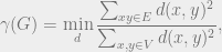
 which satisfy the
  even for
  . Certainly
  , but Bourgain’s embedding theorem (which states that every n-point metric space embeds into a Hilbert space with distortion at most
  ) also assures us that
 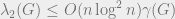 . Since we are trying to show that
  , this
  term is morally negligible. One can see the paper for a
  by taking a certain kind of all-pairs multi-commodity flow at optimality, and weighting the edges by their congestion in the optimal flow. Thus as the flow spreads out on the graph, it has the effect of “uniformizing” its geometry.
 . First, let’s restrict ourselves to vertex weighted metrics on
  , we can define the length of a path
  . Then we can define a vertex-weighted shortest-path pseudo-metric on
 is the set of all u-v paths in
![\mathsf{dist}_{\omega}(x,y) \leq [\omega(x)+\omega(y)]^2](https://s0.wp.com/latex.php?latex=%5Cmathsf%7Bdist%7D_%7B%5Comega%7D%28x%2Cy%29+%5Cleq+%5B%5Comega%28x%29%2B%5Comega%28y%29%5D%5E2&bg=eeeeee&fg=666666&s=0&c=20201002) .
.
 .
. for two well-known examples: the grid, and the complete binary tree.
 grid, we can simply take
  for all
  . Clearly
  . On the other hand, a random pair of points in the grid is
  apart, hence
  . It follows that
 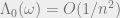 , as desired.
 , we can simply put
  and
and  for
for  . (Astute readers will guess the geometrically decreasing weights are actually the optimal choice.) In this case,
  , while all the pairs
  on opposite sides of the root have
  . It again follows that