Apparently, Bednorz and Latała have solved Talagrand’s $5,000 Bernoulli Conjecture. The conjecture concerns the supremum of a Bernoulli process.
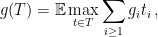
Consider a finite subset and define the value
where are i.i.d. random . This looks somewhat similar to the corresponding value
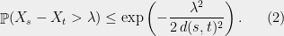
where are i.i.d. standard normal random variables. But while can be characterized (up to universal constant factors) by the Fernique-Talagrand majorizing measures theory, no similar control was known for . One stark difference between the two cases is that depends only on the distance geometry of , i.e. whenever is an affine isometry. On the other hand, can depend heavily on the coordinate structure of .
There are two basic ways to prove an upper bound on . One is via the trivial bound
The other uses the fact that the tails of Gaussians are “fatter” than those of Bernoullis.
This can be proved easily using Jensen’s inequality.
Talagrand’s Bernoulli conjecture is that can be characterized by these two upper bounds.
Bernoulli conjecture: There exists a constant such that for every , there are two subsets such that
and
Note that this is a “characterization” because given such sets and , equations (1) and (2) imply
The set controls the “Gaussian” part of the Bernoulli process, while the set controls the part that is heavily dependent on the coordinate structure.
This beautiful problem finally appears to have met a solution. While I don’t know of any applications yet in TCS, it does feel like something powerful and relevant.
We will now prove Talagrand’s majorizing measures theorem, showing that the generic chaining bound is tight for Gaussian processes. The proof here will be a bit more long-winded than the proof from Talagrand’s book, but also (I think), a bit more accessible as well. Most importantly, we will highlight the key idea with a simple combinatorial argument.
Theorem 1 Let be a Gaussian process, and let be a sequence of subsets such that and for . Then,
In order to make things slightly easier to work with, we look at an essentially equivalent way to state (1). Consider a Gaussian process and a sequence of increasing partitions of , where increasing means that is a refinement of for . Say that such a sequence is admissible if and for all . Also, for a partition and a point , we will use the notation for the unique set in which contains .
By choosing to be any set of points with one element in each piece of the partition , (1) yields,
We can now state our main theorem, which shows that this is essentially the only way to bound .
Theorem 2 There is a constant such that for any Gaussian process , there exists an admissible sequence which satisfies,
Theorem 3 For some constants and , the following holds. Suppose is a Gaussian process, and let be such that for . Then,
We will use only Theorem 3 and the fact that whenever to prove Theorem 2 (so, in fact, Theorem 2 holds with replaced by more general functionals satisfying an inequality like (4)).
The partitioning scheme
First, we will specify the partitioning scheme to form an admissible sequence , and then we will move on to its analysis. As discussed in earlier posts, we may assume that is finite. Every set will have a value associated with it, such that is always an upper bound on the radius of the set , i.e. there exists a point such that .
Initially, we set and . Now, we assume that we have constructed , and show how to form the partition . To do this, we will break every set into at most pieces. This will ensure that
Let be the constant from Theorem 3. Put , and let . We partition into pieces as follows. First, choose which maximizes the value
Then, set . We put .
A remark: The whole idea here is that we have chosen the “largest possible piece,” (in terms of -value), but we have done this with respect to the ball, while we cut out the ball. The reason for this will not become completely clear until the analysis, but we can offer a short explanation here. Looking at the lower bound (4), observe that the balls are disjoint under the assumptions, but we only get “credit” for the balls. When we apply this lower bound, it seems that we are throwing a lot of the space away. At some point, we will have to make sure that this thrown away part doesn’t have all the interesting stuff! The reason for our choice of vs. is essentially this: We want to guarantee that if we miss the interesting stuff at this level, then the previous level took care of it. To have this be the case, we will have to look forward (a level down), which (sort of) explains our choice of optimizing for the ball.
Now we continue in this fashion. Let be the remaining space after we have cut out pieces. For , choose to maximize the value
For , set , and put .
So far, we have been chopping the space into smaller pieces. If for some , we have finished our construction of . But maybe we have already chopped out pieces, and still some remains. In that case, we put , i.e. we throw everything else into . Since we cannot reduce our estimate on the radius, we also put .
We continue this process until is exhausted, i.e. eventually for some large enough, only contains singletons. This completes our description of the partitioning.
The tree
For the analysis, it will help to consider our partitioning process as having constructed a tree (in the most natural way). The root of the the tree is the set , and its children are the sets of , and so on. Let’s call this tree . It will help to draw and describe in a specific way. First, we will assign values to the edges of the tree. If and is a child of (i.e., and ), then the edge is given value:
If we define the value of a root-leaf path in as the sum of the edge lengths on that path, then for any ,
simply using .
Thus in order to prove Theorem 2, which states that for some ,
it will suffice to show that for some (other) constant , for any root-leaf path in , we have
Before doing this, we will fix a convention for drawing parts of . If a node has children , we will draw them from left to right. We will call an edge a right turn and every other edge will be referred to as a left turn. Note that some node may not have any right turn coming out of it (if the partitioning finished before the last step). Also, observe that along a left turn, the radius always drops by a factor of , while along a right turn, it remains the same.
We now make two observations about computing the value up to a universal constant.
Observation (1): In computing the value of a root-leaf path , we only need to consider right turns.
To see this, suppose that we have a right turn followed by a consecutive sequence of left turns. If the value of the right turn is , then the value of the following sequence of left turns is, in total, at most
In other words, because the radius decreases by a factor of along every left turn, their values decrease geometrically, making the whole sum comparable to the preceding right turn. (Recall that , so indeed the sum is geometric.)
If the problem of possibly of having no right turn in the path bothers you, note that we could artificially add an initial right turn into the root with value . This is justified since always holds. A different way of saying this is that if the path really contained no right turn, then its value is , and we can easily prove (6).
Observation (2): In computing the value of a root-leaf path , we need only consider the last right turn in any consecutive sequence of right turns.
Consider a sequence of consecutive right turns, and the fact that the radius does not decrease. The values (taking away the factor) look like . In other words, they are geometrically increasing, and thus using only the last right turn in every sequence, we only lose a constant factor.
We will abbreviate last right turn to LRT, and write to denote the value of , just counting last right turns. By the two observations, to show (6) (and hence finish the proof), it suffices to show that, for every root-leaf path in ,
The analysis
Recall that our tree has values on the edges, defined in (5). We will also put some natural values on the nodes. For a node (which, recall, is just a subset ), we put . So the edges have values and the nodes have values. Thus given any subset of nodes and edges in , we can talk about the value of the subset, which will be the sum of the values of the objects it contains. We will prove (7) by a sequence of inequalities on subsets.
Fix a root-leaf path , for which we will prove (7). Let’s prove the fundamental inequality now. We will consider two consecutive LRTs along . (If there is only one LRT in , then we are done by the preceding remarks.) See the figure below. The dashed lines represent a (possibly empty) sequence of left turns and then right turns. The two LRTs are marked.
We will prove the following inequality, which is the heart of the proof. One should understand that the inequality is on the values of the subsets marked in red. The first subset contains two nodes, and the second contains two nodes and an edge.
Figure A.
With this inequality proved, the proof is complete. Let’s see why. We start with the first LRT. Since for any node in , we have the inequality:
This gets us started. Now we apply the inequality of Figure A repeatedly to each pair of consecutive LRTs in the path . What do we have when we’ve exhausted the path ? Well, precisely all the LRTs in are marked, yielding , as desired.
The LRT inequality
Now we are left to prove the inequality in Figure A. First, let’s label some of the nodes. Let , and suppose that . The purple values are not the radii of the corresponding nodes, but they are upper bounds on the radii, recalling that along every left turn, the radius decreases by a factor of . Since there are at least two left turns in the picture, we get a upper bound on the radius of .
Part of the inequality is easy: We have since . So we can transfer the red mark from to . We are thus left to prove that
This will allow us to transfer the red mark from to the LRT coming out of and to .
When was partitioned into pieces, this was by our greedy partitioning algorithm using centers . Since we cut out the ball around each center, we have for all . Applying the Sudakov inequality (Theorem 3), we have
where the last line follows from the greedy manner in which the ‘s were chosen.
But now we claim that
This follows from two facts. First, (since actually). Secondly, the radius of is at most ! But was chosen to maximize the value of over all balls of radius , so in particular its -value is at least that of the ball containing .
Combining (9) and the preceding inequality, we prove (8), and thus that the inequality of Figure A is valid. This completes the proof.
In order to prove that the chaining argument is tight, we will need some additional properties of Gaussian processes. For the chaining upper bound, we used a series of union bounds specified by a tree structure. As a first step in producing a good lower bound, we will look at a way in which the union bound is tight.
Theorem 1 (Sudakov inequality) For some constant , the following holds. Let be a Gaussian process such that for every distinct , we have . Then,
The claim is an elementary calculation for a sequence of i.i.d. random variables (i.e. ). We will reduce the general case to this one using Slepian’s comparison lemma.
Lemma 2 (Slepian’s Lemma) Let and be two Gaussian processes such that for all ,
Then .
There is a fairly elementary proof of Slepian’s Lemma (see, e.g. the Ledoux-Talagrand book), if one is satisfied with the weaker conclusion , which suffices for our purposes.
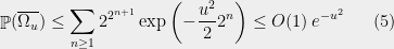
To see that Lemma 2 yields Theorem 1, take a family with for all and consider the associated variables where is a family of i.i.d. random variables. It is straightforward to verify that (1) holds, hence by the lemma, , and the result follows from the i.i.d. case.
The Sudakov inequality gives us “one level” of a lower bound; the following strengthening will allow us to use it recursively. If we have a Gaussian process and , we will use the notation
For and , we also use the notation
Here is the main theorem of this post; its statement is all we will require for our proof of the majorizing measures theorem:
Theorem 3 For some constants and , the following holds. Suppose is a Gaussian process, and let be such that for . Then,
The proof of the preceding theorem relies on the a strong concentration property for Gaussian processes. First, we recall the classical isoperimetric inequality for Gaussian space (see, for instance, (2.9) here).
We remind the reader that for a function ,
Theorem 4 Let , and let , where is the standard -dimensional Gaussian measure. Then,
Using this, we can prove the following remarkable fact.
Theorem 5 Let be a Gaussian process, then
A notable aspect of this statement is that only the maximum variance affects the concentration, not the number of random variables. We now prove Theorem 5 using Theorem 4.
Proof: We will prove it in the case , but of course our bound is independent of . The idea is that given a Gaussian process , we can write
for , where are standard i.i.d. normals, and the matrix is a matrix of real coefficients. In this case, if is a standard -dimensional Gaussian, then the vector is distributed as .
If we put , then Theorem 4 yields (3) as long as . It is easy to see that
But is just the maximum norm of any row of , and the norm of row is
Using this theorem, we are ready to prove Theorem 3. I will only give a sketch here, but filling in the details is not too difficult.
Assume that the conditions of Theorem 3 hold. Pick an arbitrary , and recall that we can write
so we could hope that for some , we simultaneously have , yielding
The problem, of course, is that the events we are discussing are not independent.
This is where Theorem 5 comes in. For any , all the variances of the variables are bounded by . This implies that we can choose a constant such that
So, in fact, we can expect that none of the random variables will deviate from its expected value by more than . Which means we can (morally) replace (4) by
In the last post, we considered a Gaussian process and were trying to find upper bounds on the quantity . We saw that one could hope to improve over the union bound by clustering the points and then taking mini union bounds in each cluster.
Hierarchical clustering
To specify a clustering, we’ll take a sequence of progressively finer approximations to our set . First, recall that we fixed , and we have used the observation that .
Now, assume that is finite. Write , and consider a sequence of subsets such that . We will assume that for some large enough , we have for . For every , let denote a “closest point map” which sends to the closest point in .
The main point is that we can now write, for any ,
This decomposition is where the term “chaining” arises, and now the idea is to bound the probability that is large in terms of the segments in the chain.
What should look like?
One question that arises is how we should think about choosing the approximations . We are trading off two measures of quality: The denser is in the set (or, more precisely, in the set ) the smaller the variances of the segments will be. On the other hand, the larger is, the more segments we’ll have to take a union bound over.
So far, we haven’t used any property of our random variables except for the fact that they are centered. To make a more informed decision about how to choose the sets , let’s recall the classical Gaussian concentration bound.
Lemma 1 For every and ,
This should look familiar: is a mean-zero Gaussian with variance .
Now, a first instinct might be to choose the sets to be progressively denser in . In this case, a natural choice would be to insist on something like being a -net in . If one continues down this path in the right way, a similar theory would develop. We’re going to take a different route and consider the other side of the tradeoff.
Instead of insisting that has a certain level of accuracy, we’ll insist that is at most a certain size. Should we require or , or use some other function? To figure out the right bound, we look at (2). Suppose that are i.i.d. random variables. In that case, applying (2) and a union bound, we see that to achieve
we need to select . If we look instead at points instead of points, the bound grows to . Thus we can generally square the number of points before the union bound has to pay a constant factor increase. This suggests that the right scaling is something like . So we’ll require that for all .
The generic chaining
This leads us to the generic chaining bound, due to Fernique (though the formulation we state here is from Talagrand).
Theorem 2 Let be a Gaussian process, and let be a sequence of subsets such that and for . Then,
Proof: As before, let denote the closest point map and let . Using (2), for any , , and , we have
Now, the number of pairs can be bounded by , so we have
Theorem 1.2 gives us a fairly natural way to upper bound the expected supremum using a hierarchical clustering of . Rather amazingly, as we’ll see in the next post, this upper bound is tight. Talagrand’s majorizing measure theorem states that if we take the best choice of in Theorem 1.2, then the upper bound in (3) is within a constant factor of .
While I’ll eventually try to give an overview of this connection, I first wanted to discuss how majorizing measures are used to control Gaussian processes. In the next few posts, I’ll attempt to give an idea of how this works. I have very little new to offer over what Talagrand has already written; in particular, I will be borrowing quite heavily from Talagrand’s book (which you might read instead).
Gaussian processes
Consider a Gaussian process for some index set . This is a collection of jointly Gaussian random variables, meaning that every finite linear combination of the variables has a Gaussian distribution. We will additionally assume that the process is centered, i.e. for all .
It is well-known that such a process is completely characterized by the covariances . For , consider the canonical distance,
which forms a metric on . (Strictly speaking, this is only a pseudometric since possibly even though and are distinct random variables, but we’ll ignore this.) Since the process is centered, it is completely specified by the distance , up to translation by a Gaussian (e.g. the process will induce the same distance for any ).
A concrete perspective
If the index set is countable, one can describe every such process in the following way. Let be a sequence of i.i.d. standard Gaussians, let , and put
In this case, it is easy to check that for . (That this construction is universal follows from the fact that every two separable Hilbert spaces are isomorphic.)
Random projections
If is finite, then we can think of for some . In this case, if is a standard -dimensional Gaussian, then
and we can envision the process as the projection of onto a uniformly random direction.
Studying the maxima
We will be concerned primarily with the value,
(I.e. the expected value of the extremal node circled above.) One may assume that is finite without losing any essential ingredient of the theory, in which case the supremum can be replaced by a maximum. Note that we are studying the tails of the process. Dealing with these extremal values is what makes understanding the above quantity somewhat difficult.
As some motivation for the classical study of this quantity, one has the following.
Theorem 1 For a separable Gaussian process , the following two assertions are equivalent.
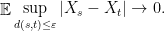
The map is uniformly continuous (as a map from to with probability one.
As ,
However, from our viewpoint, the quantitative study of in terms of the geometry of will play the fundamental role.
Bounding the sup
We will concentrate first on finding good upper bounds for . Toward this end, fix some , and observe that
Since is a non-negative random variable, we can write
and concentrate on finding upper bounds on the latter probabilities.
Improving the union bound
As a first step, we might write
While this bound is decent if the variables are somewhat independent, it is rather abysmal if the variables are clustered.
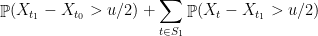
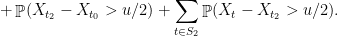
Since the variables in, e.g. , are highly correlated (in the “geometric” language, they tend to project close together on a randomly chosen direction), the union bound is overkill. It is natural to choose representatives and . We can first bound and , and then bound the intra-cluster values and . This should yield better bounds as the diameter of and are hopefully significantly smaller than the diameter of .
Formally, we have
Of course, there is no reason to stop at one level of clustering, and there is no reason that we should split the contribution evenly. In the next post, we’ll see the “generic chaining” method which generalizes and formalizes our intuition about improving the union bound. In particular, we’ll show that every hierarchical clustering of our points offers some upper bound on .


such that for every
such that


 be a Gaussian process, and let
  be a sequence of subsets such that
  and
and  for
for  . Then,
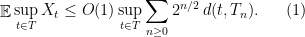
 of
of  is a refinement of
  for
for  . Say that such a sequence
  is admissible if
  and
and  for all
  and a point
  , we will use the notation
  for the unique set in
  .
. to be any set of points with one element in each piece of the partition
 .
. such that for any Gaussian process
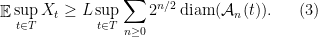
 , we defined
 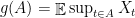 , and in the last post,
  and
and  , the following holds. Suppose
  be such that
  for
for  . Then,
 whenever
  to prove Theorem
  will have a value
  associated with it, such that
  , i.e. there exists a point
  such that
  .
. . Now, we assume that we have constructed
  pieces. This will ensure that
 be the constant from Theorem
  , and let
  . We partition
  pieces as follows. First, choose
  which maximizes the value
 . We put
  .
. -value), but we have done this with respect to the
  ball, while we cut out the
  ball. The reason for this will not become completely clear until the analysis, but we can offer a short explanation here. Looking at the lower bound
  are disjoint under the assumptions, but we only get “credit” for the
  balls. When we apply this lower bound, it seems that we are throwing a lot of the space away. At some point, we will have to make sure that this thrown away part doesn’t have all the interesting stuff! The reason for our choice of
  be the remaining space after we have cut out
  pieces. For
  , choose
  to maximize the value
 , set
, set  , and put
  .
. for some
  pieces, and still some remains. In that case, we put
  , i.e. we throw everything else into
  . Since we cannot reduce our estimate on the radius, we also put
  .
. large enough,
  , and so on. Let’s call this tree
  . It will help to draw and describe
  is a child of
  and
and  ), then the edge
  is given value:
 and
and 
 .
.

 , we will draw them from left to right. We will call an edge
  a right turn and every other edge will be referred to as a left turn. Note that some node
 up to a universal constant.
 , then the value of the following sequence of left turns is, in total, at most
 . This is justified since
  always holds. A different way of saying this is that if the path really contained no right turn, then its value is
  , and we can easily prove
  factor) look like
  . In other words, they are geometrically increasing, and thus using only the last right turn in every sequence, we only lose a constant factor.
 to denote the value of
 ), we put
  . So the edges have values and the nodes have values. Thus given any subset of nodes and edges in

 for any node
  in
in  , we have the inequality:
 ? Well, precisely all the LRTs in
  , as desired.
 .
.
 since
since  . So we can transfer the red mark from
  . We are thus left to prove that
 . Since we cut out the
  for all
 ‘s were chosen.
 (since
  actually). Secondly, the radius of
  was chosen to maximize the value of
  over all balls of radius
  , the following holds. Let
  be a Gaussian process such that for every distinct
  , we have
  . Then,
 random variables
  (i.e.
(i.e.  ). We will reduce the general case to this one using Slepian’s comparison lemma.
 be two Gaussian processes such that for all
 .
.  , which suffices for our purposes.
 and consider the associated variables
  where
where  is a family of i.i.d.
  , and the result follows from the i.i.d. case.
 , we will use the notation
 and
and  , we also use the notation
 and
and  , the following holds. Suppose
  be such that
  for
for  . Then,

 ,
,
 , where
  is the standard
  -dimensional Gaussian measure. Then,

 , but of course our bound is independent of
  , we can write
 , where
  are standard i.i.d. normals, and the matrix
  is a matrix of real coefficients. In this case, if
  is a standard
  is distributed as
  .
. , then Theorem
  . It is easy to see that
 is just the maximum
  norm of any row of
  , and the
  is
is 


 , and recall that we can write

 achieves this. By definition,
 , we simultaneously have
  , yielding
 are bounded by
  . This implies that we can choose a constant
  such that
 random variables
  will deviate from its expected value by more than
 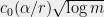 . Which means we can (morally) replace
 , the error term is absorbed.
  . We saw that one could hope to improve over the union bound by clustering the points and then taking mini union bounds in each cluster.
 . First, recall that we fixed
  .
. , and consider a sequence of subsets
  such that
  . We will assume that for some large enough
  for
for  . For every
  , let
, let  denote a “closest point map” which sends
  to the closest point in
  .
.
 is large in terms of the segments in the chain.
 look like?
  ) the smaller the variances of the segments
  will be. On the other hand, the larger
  ,
, 
 is a mean-zero Gaussian with variance
  .
. -net in
  or
or  , or use some other function? To figure out the right bound, we look at
  are i.i.d.
 . If we look instead at
  points instead of
  . Thus we can generally square the number of points before the union bound has to pay a constant factor increase. This suggests that the right scaling is something like
  . So we’ll require that
  for all
  .
. be a sequence of subsets such that
  and
and  for
for 
 , we have
 can be bounded by
  , so we have

 , since we get geometrically decreasing summands.
 occurs, then
  . Thus
  ,
, 


 .
. for all
  . For
. For  , consider the canonical distance,
 even though
  and
and  are distinct random variables, but we’ll ignore this.) Since the process is centered, it is completely specified by the distance
  , up to translation by a Gaussian (e.g. the process
  will induce the same distance for any
  ).
). be a sequence of i.i.d. standard Gaussians, let
 for
for  for some
  . In this case, if


 is uniformly continuous (as a map from
  to
to  with probability one.
 ,
,
 in terms of the geometry of
  . Toward this end, fix some
 is a non-negative random variable, we can write
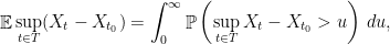

 are somewhat independent, it is rather abysmal if the variables are clustered.
 , are highly correlated (in the “geometric” language, they tend to project close together on a randomly chosen direction), the union bound is overkill. It is natural to choose representatives
  and
and  . We can first bound
  and
and  , and then bound the intra-cluster values
  and
and  . This should yield better bounds as the diameter of
  are hopefully significantly smaller than the diameter of
 evenly. In the next post, we’ll see the “generic chaining” method which generalizes and formalizes our intuition about improving the union bound. In particular, we’ll show that every hierarchical clustering of our points offers some upper bound on
  .
.