At STOC 2010 last week, Talagrand gave a presentation on some of his favorite open problems, which included a quick review of Gaussian processes and the majorizing measures theory. In joint work with Jian Ding and Yuval Peres, we recently showed how the cover time of graphs can be characterized by majorizing measures.
While I’ll eventually try to give an overview of this connection, I first wanted to discuss how majorizing measures are used to control Gaussian processes. In the next few posts, I’ll attempt to give an idea of how this works. I have very little new to offer over what Talagrand has already written; in particular, I will be borrowing quite heavily from Talagrand’s book (which you might read instead).
Gaussian processes
Consider a Gaussian process for some index set
. This is a collection of jointly Gaussian random variables, meaning that every finite linear combination of the variables has a Gaussian distribution. We will additionally assume that the process is centered, i.e.
for all
.
It is well-known that such a process is completely characterized by the covariances . For
, consider the canonical distance,
which forms a metric on . (Strictly speaking, this is only a pseudometric since possibly
even though
and
are distinct random variables, but we’ll ignore this.) Since the process is centered, it is completely specified by the distance
, up to translation by a Gaussian (e.g. the process
will induce the same distance for any
).
A concrete perspective
If the index set is countable, one can describe every such process in the following way. Let
be a sequence of i.i.d. standard Gaussians, let
, and put
In this case, it is easy to check that for
. (That this construction is universal follows from the fact that every two separable Hilbert spaces are isomorphic.)
Random projections
If is finite, then we can think of
for some
. In this case, if
is a standard
-dimensional Gaussian, then
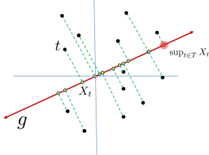
and we can envision the process as the projection of onto a uniformly random direction.
Studying the maxima
We will be concerned primarily with the value,
(I.e. the expected value of the extremal node circled above.) One may assume that is finite without losing any essential ingredient of the theory, in which case the supremum can be replaced by a maximum. Note that we are studying the tails of the process. Dealing with these extremal values is what makes understanding the above quantity somewhat difficult.
As some motivation for the classical study of this quantity, one has the following.
Theorem 1 For a separable Gaussian process
, the following two assertions are equivalent.
- The map
is uniformly continuous (as a map from
to
with probability one.
- As
,
However, from our viewpoint, the quantitative study of in terms of the geometry of
will play the fundamental role.
Bounding the sup
We will concentrate first on finding good upper bounds for . Toward this end, fix some
, and observe that
Since is a non-negative random variable, we can write
and concentrate on finding upper bounds on the latter probabilities.
Improving the union bound
As a first step, we might write
While this bound is decent if the variables are somewhat independent, it is rather abysmal if the variables are clustered.
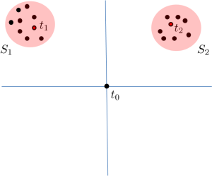
Since the variables in, e.g. , are highly correlated (in the “geometric” language, they tend to project close together on a randomly chosen direction), the union bound is overkill. It is natural to choose representatives
and
. We can first bound
and
, and then bound the intra-cluster values
and
. This should yield better bounds as the diameter of
and
are hopefully significantly smaller than the diameter of
.
Formally, we have
Of course, there is no reason to stop at one level of clustering, and there is no reason that we should split the contribution evenly. In the next post, we’ll see the “generic chaining” method which generalizes and formalizes our intuition about improving the union bound. In particular, we’ll show that every hierarchical clustering of our points offers some upper bound on
.


Thank you! Even though I knew about the chaining technique, but still your post helped me to have a better intuition. I liked the cluster diagram!
thank you very much, for your comments , your diagramms very helpful!!