The pseudorandom subspace problem

In this post, I will talk about the existence and construction of subspaces of $\ell_1^N$ which are “almost Euclidean.” In the next few, I’ll discuss the relationship between such subspaces, compressed sensing, and error-correcting codes over the reals.

A good starting point is Dvoretzky’s theorem:

For every $N \in \mathbb N$ and $\varepsilon > 0$ , the following holds. Let $|\cdot|$ be the Euclidean norm on $\mathbb R^N$ , and let $\|\cdot\|$ be an arbitrary norm. Then there exists a subspace $X \subseteq \mathbb R^N$ with $\mathrm{dim}(X) \geq c(\varepsilon) \log N$ , and a number $A > 0$ so that for every $x\in X$ ,

$\displaystyle A|x| \leq \|x\| \leq (1+\varepsilon) A |x|$ .

Here, $c(\varepsilon) > 0$ is a constant that depends only on $\varepsilon$ .

The theorem as stated is due to Vitali Milman, who gave the (optimal) dependence of $\log N$ on the dimension of $X$ , and proved that the above fact actually holds with high probability when $X$ is chosen uniformly at random from all subspaces of this dimension. In other words, for $d \approx \log N$ , a random $d$ -dimensional subspace of an arbitrary $N$ -dimensional normed space is almost Euclidean. Milman’s proof was one of the starting points for the “local theory” of Banach spaces, which views Banach spaces through the lens of sequences of finite-dimensional subspaces whose dimension goes to infinity. It’s a very TCS-like philosophy; see the book of Milman and Schechtman.

One can associate to any norm its unit ball $B = \left\{ x \in \mathbb R^N : \|x\| \leq 1 \right\}$ , which will be a centrally symmetric convex body. Thus we can restate Milman’s proof of Dvoretzky’s theorem geometrically: If $B$ is an arbitrary convex body, and $H$ is a random $c(\varepsilon) \log N$ -dimensional hyperplane through the origin, then with high probability, $B \cap H$ will almost be a Euclidean ball. This is quite surprising if one starts, for instance, with a polytope like the unit cube or the cross polytope. The intersection $B \cap H$ is again a polytope, but which is approximated closely by a smooth ball. Here’s a pictorial representation lifted from a talk I once gave:

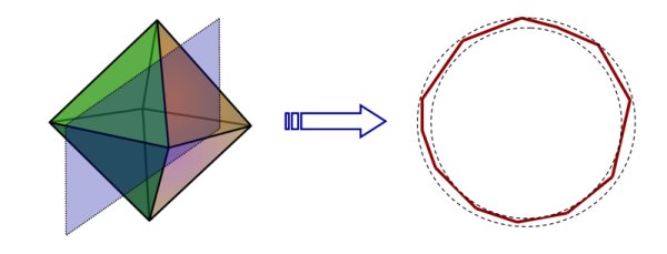
(Note: Strictly speaking, the intersection will only be an ellipsoid, and one might have to pass to a subsection to actually get a Euclidean sphere.)

Euclidean subspaces of $\ell_1^N$ and Error-Correcting Codes.

It is not too difficult to see that the dependence $\mathrm{dim}(X) \approx \log N$ is tight when we consider $\mathbb R^N$ equipped with the $\ell_\infty$ norm (see e.g. Claim 3.10 in these notes), but rather remarkably, results of Kasin and Figiel, Lindenstrauss, and Milman show that if we consider the $\ell_1$ norm, we can find Euclidean subspaces of proportional dimension, i.e. $\mathrm{dim}(X) \approx N$ .

For any $x \in \mathbb R^N$ , Cauchy-Schwarz gives us

$\|x\|_2 \leq \|x\|_1 \leq \sqrt{N} \|x\|_2.$

To this end, for a subspace $X \subseteq \mathbb R^N$ , let’s define

$\displaystyle \Delta(X) = \max_{0 \neq x \in \mathbb R^N} \frac{\sqrt{N} \|x\|_2}{\|x\|_1},$

which measures how well-spread the $\ell_2$ -mass is among the coordinates of vectors $x \in X$ . For instance, if $\Delta(X) = O(1)$ , then every non-zero $x \in \mathbb X$ has at least $\Omega(N)$ non-zero coordinates (because $\|x\|_1 \leq \sqrt{|\mathrm{supp}(x)|} \|x\|_2$ ). This has an obvious analogy with the setting of linear error-correcting codes, where one would like the same property from the kernel of the check matrix. Over the next few posts, I’ll show how such subspaces actually give rise to error-correcting codes over $\mathbb R$ that always have efficient decoding algorithms.

The Kasin and Figiel-Lindenstrauss-Milman results actually describe two different regimes. Kasin shows that for every $\eta > 0$ , there exists a subspace $X \subseteq \mathbb R^N$ with $\dim(X) \geq (1-\eta) N$ , and $\Delta(X) = O_{\eta}(1)$ . The FLM result shows that for every $\varepsilon > 0$ , one can get $\Delta(X) \leq 1 + \varepsilon$ and $\dim(X) \geq \Omega_{\varepsilon}(N)$ . In coding terminology, the former approach maximizes the rate of the code, while the latter maximizes the minimum distance. In this post, we will be more interested in Kasin’s “nearly full dimensional” setting, since this has the most relevance to sensing and coding. Work of Indyk (see also this) shows that the “nearly isometric” setting is useful for applications in high-dimensional nearest-neighbor search.

The search for explicit constructions

Both approaches show that the bounds hold for a random subspace of the proper dimension (where “random” can mean different things;we’ll see one example below). In light of this, many authors have asked whether there are explicit constructions of such subspaces exist, see e.g. Johnson and Schechtman (Section 2.2), Milman (Problem 8), and Szarek (Section 4). As I’ll discuss in future posts, this would also yield explicit constructions of codes over the reals, and of compressed sensing matrices.

Depending on the circles you run in, “explicit” can mean different things. Let’s fix a TCS-style definition: An explicit construction means a deterministic algorithm which, give $N$ as input, outputs a description of a subspace $X$ (e.g. in the form of a set of basis vectors), and runs in time $\mathrm{poly}(N)$ . Fortunately, the constructions I’ll discuss later will satisfy just about everyone’s sense of explicitness.

In light of the difficulty of obtaining explicit constructions, people have started looking at weaker results and partial derandomizations. One starting point is Kasin’s method of proof: He shows, for instance, that if one chooses a uniformly random $N/2 \times N$ sign matrix $A$ (i.e. one whose entries are chosen independently and uniformly from $\{-1,1\}$ ), then with high probability, one has $\Delta(\mathrm{ker}(A)) = O(1)$ . Of course this bears a strong resemblance to random parity check codes. Clearly we also get $\dim(\mathrm{ker}(A)) \geq N/2$ .

In work of Guruswami, myself, and Razborov, we show that there exist explicit $N/2 \times N$ sign matrices $A$ for which $\Delta(\mathrm{ker}(A)) \leq (\log N)^{O(\log \log \log N)}$ (recall that the trivial bound is $\Delta(\cdot) \leq \sqrt{N}$ ). Our approach is inspired by the construction and analysis of expander codes. Preceding our work, Artstein-Avidan and Milman pursued a different direction, by asking whether one can reduce the dependence on the number of random bits from the trivial $O(N^2)$ bound (and still achieve $\Delta(\mathrm{ker}(A)) = O(1)$ ). Using random walks on expander graphs, they showed that one only needs $O(N \log N)$ random bits to construct such a subspace. Lovett and Sodin later reduced this dependency to $O(N)$ . (Indyk’s approach based on Nisan’s pseudorandom generator can also be used to get $O(N \log^2 N)$ .) In upcoming work with Guruswami and Wigderson, we show that the dependence can be reduced to $O(N^{\delta})$ for any $\delta > 0$ .

Kernels of random sign matrices

It makes sense to end this discussion with an analysis of the random case. We will prove that if $A$ is a random $N/2 \times N$ sign matrix (assume for simplicity that $N$ is even), then with high probability $\Delta(\mathrm{ker}(A)) = O(1)$ . It might help first to recall why a uniformly random $N/2 \times N$ matrix $B$ with $\{0,1\}$ entries is almost surely the check matrix of a good linear code.

Let $\mathbb F_2 = \{0,1\}$ be the finite field of order 2. We would like to show that, with high probability, there does not exist a non-zero vector $x \in \mathbb F_2^N$ with hamming weight $o(N)$ , and which satisfies $Bx=0$ (this equation is considered over $\mathbb F_2$ ). The proof is simple: Let $B_1, B_2, \ldots, B_{N/2}$ be the rows of $B$ . If $x \neq 0$ , then $\Pr[\langle B_i, x \rangle = 0] \leq \frac12.$ Therefore, for any non-zero $x$ , we have

$\Pr[Bx = 0] \leq 2^{-N/2}.$ (**)

On the other hand, for $\delta > 0$ small enough, there are fewer than $2^{N/2}$ non-zero vectors of hamming weight at most $\delta N$ , so a union bound finishes the argument.

The proof that $\Delta(\mathrm{ker}(A)) = O(1)$ proceeds along similar lines, except that we can no longer take a naive union bound since there are now infinitely many “bad” vectors. Of course the solution is to take a sufficiently fine discretization of the set of bad vectors. This proceeds in three steps:

If $x$ is far from $\mathrm{ker}(A)$ , then any $x'$ with $\|x-x'\|_2$ small is also far from $\mathrm{ker}(A)$ .
Any fixed vector $x \in \mathbb R^N$ with $\|x\|_2 = 1$ is far from $\mathrm{ker}(A)$ with very high probability. This is the analog of (**) in the coding setting.
There exists a small set of vectors that well-approximates the set of bad vectors.

Combining (1), (2), and (3) we will conclude that every bad vector is far from the kernel of $A$ (and, in particular, not contained in the kernel).

To verify (1), we need to show that almost surely the operator norm $\|A\| = \max \left\{ \|Ax\|_2 : \|x\|_2 = 1\right\}$ is small, because if we define

$\mathrm{dist}(x, \mathrm{ker}(A)) = \min_{y \in \mathrm{ker}(A)} \|x-y\|_2$ ,

then

$\mathrm{dist}(x', \mathrm{ker}(A)) \geq \mathrm{dist}(x,\mathrm{ker}(A)) - \|A\| \cdot \|x-x'\|_2$

In order to proceed, we first need a tail bound on random Bernoulli sums, which follows immediately from Hoeffding’s inequality.

Lemma 1: If $v \in \mathbb R^k$ and $X \in \{-1,1\}^k$ is chosen uniformly at random, then

$\displaystyle \Pr\left[|\langle v, X \rangle| \geq t\right] \leq 2 \exp\left(\frac{-t^2}{2 \|v\|_2^2}\right)$

In particular, for $y \in \mathbb R^{N/2}$ and $x \in \mathbb R^N$ , we have $\langle y, Ax \rangle = \sum_{i=1}^{N/2} \sum_{j=1}^N A_{ij} y_i x_j$ . We conclude that if we take $\|x\|_2 = 1$ and $\|y\|_2 = 1$ , then

$\Pr\left[ |\langle y, Ax \rangle| \geq t \sqrt{2N}\right] \leq 2 \exp\left(-t^2 N\right),$ (4)

observing that $\sum_{i,j} y_i^2 x_j^2 = 1$ , and applying Lemma 1. Now we can prove that $\|A\|$ is usually not too big.

Theorem 1: If $A$ is a random $N/2 \times N$ sign matrix, then

$\Pr[\|A\| \geq 10 \sqrt{N}] \leq 2 e^{-6N}$ .

Proof:

For convenience, let $m = N/2$ , and let $\Gamma_m$ and $\Gamma_N$ be $(1/3)$ -nets on the unit spheres of $\mathbb R^m$ and $\mathbb R^N$ , respectively. In other words, for every $x \in \mathbb R^m$ with $\|x\|_2 = 1$ , there should exist a point $x' \in \Gamma_m$ for which $\|x-x'\|_2 \leq 1/3$ , and similarly for $\Gamma_N$ . It is well-known that one can choose such nets with $|\Gamma_m| \leq 7^m$ and $|\Gamma_N| \leq 7^N$ (see, e.g. the book of Milman and Schechtman mentioned earlier).

So applying (4) and a union bound, we have

$\displaystyle \Pr\left[\exists y \in \Gamma_m, x \in \Gamma_N\,\, |\langle y, Ax \rangle| \geq 3\sqrt{2N}\right] \leq 2 |\Gamma_m| |\Gamma_N| \exp(-9N) \leq 2 \exp(-6N).$

So let’s assume that no such $x \in \Gamma_N$ and $y \in \Gamma_m$ exist. Let $u \in \mathbb R^N$ and $v \in \mathbb R^m$ be arbitrary vectors with $\|u\|_2=1,\|v\|_2=1$ , and write $u = \sum_{i \geq 0} \alpha_i x_i$ and $v = \sum_{i \geq 0} \beta_i y_i$ , where $\{x_i\} \subseteq \Gamma_N$ and $\{y_i\} \subseteq \Gamma_m$ , where $|\alpha_i|, |\beta_i| \leq 3^{-i}$ (by choosing successive approximations). Then we have,

$|\langle v, A u\rangle| \leq \sum_{i,j \geq 0} 3^{-i-j} |\langle y_i, A x_i\rangle| \leq (3/2)^2 3\sqrt{2N} \leq 10 \sqrt{N}$ .

We conclude by nothing that $\|A\| = \max \left\{ |\langle u, Av \rangle| : \|u\|_2 = 1, \|v\|_2=1 \right\}$ .

This concludes the verification of (1). In the next post, we’ll see how (2) and (3) are proved.

2 thoughts on “The pseudorandom subspace problem”

aravind srinivasan says:

May 7, 2008 at 8:27 pm

hi james, welcome to the ToC blogosphere — you have started with a bang with such a detailed post! i have two questions about Dvoretzky’s Theorem as you have stated it: (i) as stated, your quantification allows A to be a function of N, the norm, and epsilon (as it is just a normalization) — is it independent of any of these — perhaps of both N and epsilon? or am i being silly here? (ii) since c(epsilon) is implicitly the infimum over all possible norms — is it known what the extremal norm is?
jrluw says:

May 7, 2008 at 9:00 pm

Hi Aravind,

Great questions. First, one can actually take $A$ to be the median of $x \mapsto \|x\|$ as $x$ ranges over the Euclidean sphere $S^{N-1}$ . (This hints at one of the core principles behind Milman’s proof: The value of $\|\cdot\|$ is sharply concentrated on $S^{N-1}$ .) In particular, $A$ does not depend on $\varepsilon$ .

The extremal space for $c(\varepsilon)$ is unknown, in fact there is still a big gap between the upper and lower bounds: $\frac{1}{\log \varepsilon^{-1}} \gtrsim c(\varepsilon) \gtrsim \frac{\varepsilon}{(\log \varepsilon^{-1})^2}$ . The upper bound comes from considering the $\ell_\infty$ norm, and the best lower bound is due to Schechtman.