In this post, I’ll discuss the relationship between multi-flows and sparse cuts in graphs, bi-lipschitz embeddings into 
Table of contents:
- The max-flow/min-cut theorem
- Multi-commodity flows and sparse cuts
- The planar multi-flow conjecture
- Bi-Lipschitz embeddings into
- The planar embedding conjecture
- Parallel geodesics and the slums of geometry
- Local rigidity and coarse differentiation
- Beyond planar graphs
The max-flow/min-cut theorem
Let 


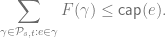
The value of the flow F is the total amount of flow sent: 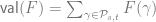


where the maximum is over all 
Multi-commodity flows and sparse cuts
We will presently be interested in multi-commodity flows (multi-flows for short), where we are given a demand function 


where the minimum is over pairs with 

Again, cuts give a natural obstruction to flows. If we define 


In fact, the gap between the two can be arbitrarily large, as witnessed by expander graphs (this rather fruitful connection will be discussed in a future post). For now, we’ll concentrate on a setting where the gap is conjectured to be at most 
The planar multi-flow conjecture
It has been conjectured that there exists a universal constant 


The conjecture first appeared in print here, but was tossed around since the publications of Linial, London, and Rabinovich and Aumann and Rabani, which recast these multi-flow/cut gaps as questions about bi-lipschitz mappings into 
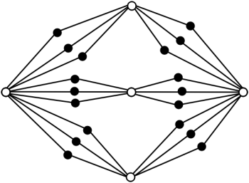
It is relatively easy to see that we cannot take 
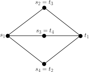
In the example, the non-zero demands are 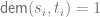


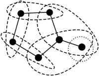
For any graph 

Bi-Lipschitz embeddings into
Consider a metric space 
![L_1 = L_1([0,1])](https://s0.wp.com/latex.php?latex=L_1+%3D+L_1%28%5B0%2C1%5D%29&bg=ffffff&fg=666666&s=0&c=20201002)


and 


We will now relate 


Here is the beautiful connection referred to previously (see this for a complete proof).
Theorem (Linial-London-Rabinovich, Aumann-Rabani): For any graph 
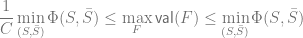
Metric obstructions. To give an idea of why the theorem is true, we mention two facts. It is rather obvious how a cut obstructs a flow. A more general type of obstruction is given by a metric 
To see why this holds, think of giving every edge 


It turns out (by linear programming duality) that in fact metrics are the correct dual objects to flows, and maximizing the left hand side of (2) over valid flows, and minimizing the right-hand side over metrics yields equality (it is also easy to see that the minimal metric is a shortest-path metric). One might ask why one continues to study cuts if they are the “wrong” dual objects. I hope to address this extensively in future posts, but the basic idea is to flip the correspondence around: minimizing 


The cut decomposition of 


Fact: Given 


Thus every 
In the 4-cycle, each cut has unit weight. The corresponding embedding into 

Two comments are in order; first, when 

The planar embedding conjecture
Using the connection with
Planar embedding conjecture: There exists a constant
By a relatively simple approximation argument in one direction, and a compactness argument in the other, one has the following equivalent conjecture.
Riemannian version: There exists a constant
Recently, Indyk and Sidiropoulos proved that if it’s true for the 2-sphere, then it’s true for every compact surface of genus 

We can now state some known results in the dual setting of embeddings. Let 

In Gromov’s language, the observable diameter of planar graph metrics is almost as large as possible (i.e. no forced concentration of Lispchitz mappings).
A classical theorem of Okamura and Seymour is stated in the embedding setting as: Let 


Finally, we mention the bound of Rao which shows that 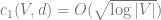


Read about the relationship with coarse differentiation after the jump.
Parallel geodesics and the slums of geometry
Of course there is an obvious parallel between taking a fixed graph
One fascinating question is how the structure of the geometries evolves as we allow the underlying graph to become more complex. It’s easy to understand the metrics supported on a path; they are all isometric to a subset of the real line. What if we allow more than one path between a pair of points?
(Consider the edges as having unit weights.) As we’ve seen, the first space embeds isometrically. It turns out that the middle graph requires distortion 

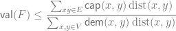
Is it possible that we can amplify this to unbounded distortion by being more clever? Consider the following operation on edges.

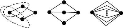
Certainly the operation preserves planarity. Starting with an initial edge, we could repeat this over and over again to get a graph like
The metrics supported on such graphs are precisely the class of shortest-path metrics on series-parallel (SP) graphs. (Although these graphs themselves do not constitute all SP graphs, by appropriately weighting them, we do exhaust all metrics supported on SP graphs.)
Gupta, Newman, Rabinovich, and Sinclair showed that all such graphs embed into
It turns out (as we showed recently with Chakrabarti, Jaffe, and Vincent) that the right answer for this class of graphs is 2. For now, we move to the lower bound.
Local rigidity and coarse differentiation
The following argument arose in joint work with P. Raghavendra.
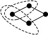
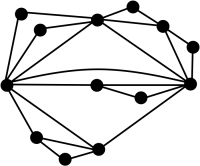
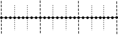
Consider 
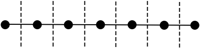
where the dotted lines represent cuts in the obvious way. The question now becomes: how stable is this property? What happens if 
Local rigidity. Instead, think of 


This is not very surprising if you’ve seen e.g. Lebesgue’s differentiation theorem or Rademacher’s theorem. But the crucial fact here is that the conclusion of Rademacher’s theorem does not hold for mappings 
![F(t) = \mathbf{1}_{[0,t]}](https://s0.wp.com/latex.php?latex=F%28t%29+%3D+%5Cmathbf%7B1%7D_%7B%5B0%2Ct%5D%7D&bg=ffffff&fg=666666&s=0&c=20201002)
![\lim_{h \to 0} h^{-1}[F(t+h)-F(t)]=\lim_{h \to 0} h^{-1} \mathbf{1}_{[t,t+h]}](https://s0.wp.com/latex.php?latex=%5Clim_%7Bh+%5Cto+0%7D+h%5E%7B-1%7D%5BF%28t%2Bh%29-F%28t%29%5D%3D%5Clim_%7Bh+%5Cto+0%7D+h%5E%7B-1%7D+%5Cmathbf%7B1%7D_%7B%5Bt%2Ct%2Bh%5D%7D&bg=ffffff&fg=666666&s=0&c=20201002)
The lower bound graphs. Recall that 

Let’s call the 


The point now is to take 


s 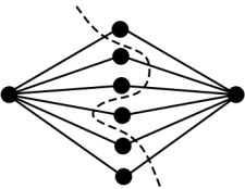 t
t
In other words, they separate 


Coarse differentiation. Finally, we move to the proof of the local rigidity statement. This is based on the coarse differentiation technique of Eskin, Fisher, and Whyte. Given a mapping 


This is a discrete sort of bounded variation. The left-hand side holds trivially from the triangle inequality, and the right-hand side says that the triangle inequality isn’t too far off, i.e. the image 
Let’s assume that 


We would like to find a segment at some scale on which
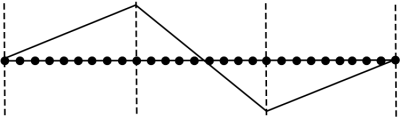
Now if
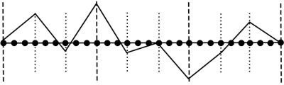
And if we fail again to find a good segment at the next scale:
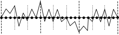
As the pictures expresses pretty clearly, every time we reveal that 
Specializing to 
Again consider the path 


If

This shows that the mapping 


So once we find a scale at which
Beyond planar graphs
The planar embedding conjecture is still open. It seems that if differentiation arguments are going to disprove it, they will have to use more than just local rigidity for paths (with some work, one can get local rigidity for grids, for instance, but then it’s hard to play around with full-blown grids without violating the topology).
If one is willing to work with a significantly more sophisticated (though still “finite-dimensional,” e.g. doubling) metric space, then a different sort of weak differentiation argument is able to show that there exists no bi-Lipschitz embedding into 

Hello admin, nice site ! Good content, beautiful design, thank !,
Amazing. Here’s a question, are there families of graphs with good separators but bad L_1-distortion?
Yes, for instance the 3-dimensional Heisenberg group mentioned at the end of the article. The results of Cheeger and Kleiner imply that grids in this group have unbounded distortion (as the size of the grid goes to infinity), but they have separators of size ~ sqrt{N}, where N is the number of points.